A Step-by-Step Protocol From METASPACE to Biological Interpretation.

Introduction

Mass spectrometry imaging (MSI) has become a very popular analytical technique for simultaneously visualizing the distribution and the relative abundance of molecules in biological tissues and microbial systems [1,2]. Among the diverse sets of molecules commonly analyzed, metabolites and lipids are among the most popular. Their study is crucial to understanding ecological interactions and biochemical processes within living organisms [3]. Research on small molecules has significant practical applications, such as natural product discovery [4], disease diagnostics [5], biofuel production, and more. Visualizing their accurate localization and characterization is critical, particularly in natural product chemistry, biomarker research, and understanding their biological activity [6]. MSI plays a crucial role in advancing these areas by providing detailed insights into the molecular distribution. However, translating MSI measurements into biological conclusions remains challenging, largely because of accurate molecular identification and interpretation by the chemical diversity of complex samples and the large number of potential molecular candidates [7].

METASPACE is a cloud‐based MSI annotation engine and knowledgebase, which is a community‐populated repository that allows researchers to investigate and putatively annotate what has been imaged by different MSI instruments [8]. At the end of 2025, METASPACE contained more than 16 000 MSI datasets submitted from all over the world. Its popularity relies on its ability to annotate and visualize metabolites [9], lipids, andN‐glycans [10] from submitted MSI datasets; the only requirement is to upload data from a high‐resolution mass spectrometer in centroided mode and in the open format imzML [11]. Once the data are submitted, an MS1‐based metabolite annotation engine processes the data and provides molecular annotations on a pseudolevel 2 (putatively annotated compounds), based on the Metabolomics Standard Initiative [12], where detected molecular formulas are annotated from selected database(s)—including customs in‐house generated databases.

To date, METASPACE includes datasets from a wide variety of instruments and samples, enabling the detection and putative identification of an extensive range of metabolites and lipid molecules. Figure1illustrates the fraction of chemical classes detected from datasets across different ionization sources. Although METASPACE facilitates the annotation, users still face a major bottleneck after annotation: efficiently summarizing, comparing, and prioritizing results across datasets or experimental conditions.

Heatmap based on METASPACE annotations illustrating detectability across chemical classes and ionization/desorption sources (Cividis colormap Ref [13]). Rows correspond to chemical classes, and columns represent ionization/desorption sources: matrix‐assisted laser desorption electrospray ionization (MALDESI), matrix‐assisted laser desorption/ionization (MALDI), laser post‐ionization MALDI (MALDI‐2), atmospheric‐Pressure (AP)‐MALDI, and desorption electrospray ionization (DESI). The color scale indicates the fraction of ions detected for each chemical class‐ionization/desorption source, with cell values reporting the fraction detected (range: 0–0.94), where 0.94 corresponds to 94% of ions detected (the maximum observed across chemical classes).

Identifying how metabolite distributions change under different conditions is one of the primary objectives in most MSI experiments, and for an untargeted metabolomics approach, these analyses require assessing the distribution of hundreds or even thousands of ions [14]. Therefore, manual inspection of ion images or spreadsheet‐based handling of annotation tables is time‐consuming, difficult to standardize, and prone to inconsistencies, particularly when multiple datasets, sample types, or acquisition methods are involved.

To address this gap, we present a practical, step‐by‐step tutorial and R‐based workflow that helps streamline the post‐METASPACE annotation of the MSI datasets. The goal of this protocol is to enable a rapid generation of interpretable results, condensed into summaries (e.g., shared vs. unique annotations and chemical class distributions), and produce refined annotation lists that can be directly used for targeted visualization and for further guidance into a deeper downstream analysis using dedicated MSI software (Figure2). This approach is intended to lower the barrier for initial biological interpretation and to improve consistency and reproducibility when working with complex MSI datasets.

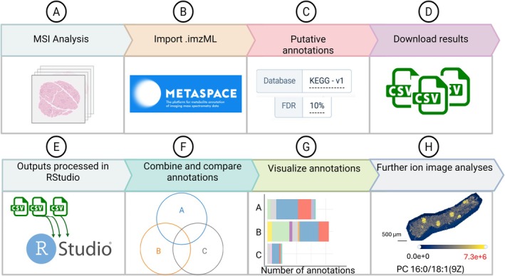
End‐to‐end workflow for MSI annotation to comparative analysis. (A–D) MSI data are acquired, converted/imported as imzML into METASPACE, evaluated across datasets, and annotation outputs are downloaded as CSV files. (E–H) CSV outputs are processed in RStudio to consolidate annotations across experiments, generate comparative summaries and visualizations, and produce a curated annotation set for targeted follow‐up, including ion‐image inspection in dedicated MSI software.

Materials and Methods

Samples from Users of the Environmental Molecular Sciences Laboratory (EMSL), from the United States National Institutes of Health Kidney Precision Medicine Project (KPMP), and published datasets available in METASPACE [15] were used as examples to showcase the use of the R‐script developed to facilitate an initial and easy inspection of datasets uploaded to METASPACE independently from the ionization source or mass analyzer used.

InExample S1,Sorghum bicolorstems were collected at two different developmental stages, 5 and 7 weeks, and metabolic profiles were analyzed in negative mode with matrix‐assisted laser desorption/ionization (MALDI) Fourier transform ion cyclotron resonance (FTICR) with a mass resolving power of 110 000 (atm/z400), usingN‐(1‐naphthyl) ethylenediamine dihydrochloride (NEDC) as the MALDI matrix, and metabolites were annotated against the KEGG [16], Core Metabolome [14], and NPA [17] databases. InExample S2, human kidney biopsies were obtained through the KPMP repository and cryosectioned at 7 μm for lipid analysis in positive mode using MALDI‐FTICR‐MSI (160 000 atm/z400), dihydroxybenzoic acid (DHB) as the matrix, and were annotated against LIPID MAPS [18], SWISS Lipid [19], and KEGG databases in METASPACE. InExample S3, published datasets of Hunter et al. were downloaded from METASPACE to showcase the utility of the R‐script for rapid inspection of annotated molecules using a different ionization source. In this study, infrared (IR) matrix‐assisted laser desorption electrospray ionization (MALDESI) was used to analyze the mouse brain with a doped solvent and/or ice matrix and without. LIPID MAPS [18] was used for annotations. For data processing and visualization, we use the free software R [20] and the integrated development environment (IDE) RStudio [21].

Step‐by‐Step Protocol

An illustration of the METASPACE cross‐dataset comparison and the datasets export workflow is shown in Figure3. Details are as follows:1Start in METASPACE. Open the project in METASPACE that contains the datasets to be analyzed and compared (Figure3A).2Select datasets for comparison. Navigate todataset overviewand select a dataset. Usedataset comparisonfeature to select the samples to compare including replicates when available (Figure3B–D). In the example shown, two sorghum stem datasets are compared.3Arrange and compare. Arrange the selected datasets in the comparison grid and clickCompare(Figure3D).4Review ion images and annotation table. A new window will display side‐by‐side ion images along with the annotation table. Each row in the table includes the ion images, the molecular formula, and the list of putative molecular features (Figure3E).5Set database and threshold. In the annotation table header, set the database and define a False Discovery Rate (FDR). An FDR of 10% is recommended by Palmer et al. [22]. To calculate the FDR, a target‐decoy approach is used to estimate how many annotations are likely incorrect. This value is dependent on the database selected; therefore, it is best to select databases most relevant to the sample type. For example, the KEGG database at 10% FDR is used for Figure3F.

6Export annotation table. Click Export to CSV to download the annotation table. Repeat this step for any additional databases that should be included in the comparison (Figure3G). Using multiple relevant databases can increase coverage; however, in targeted studies, a single specialized database may be sufficient. InExample S1, KEGG, CoreMetabolome, and Natural Product Atlas (NPA) databases were used, whereas inExample S3, only the LIPID MAPS database was selected because lipids were the primary molecular target for this study [15].

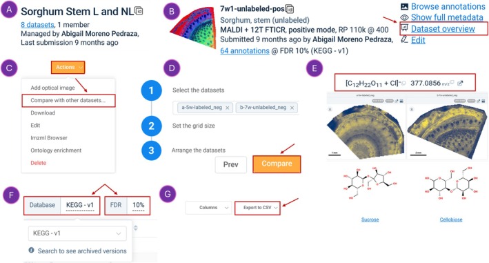
METASPACE step‐by‐step workflow for cross‐dataset comparison, using sorghum stem data as the comparison. (A) Select the project (here: Sorghum Stem L and NL). (B) Choose a dataset and open Dataset overview (red box). (C) From the Actions menu, select Compare with other datasets(red box). (D) In the Datasets comparison view, select the datasets, arrange them for side‐by‐side display, and click Compare. (E) Example annotation showing a molecular formula assignment (red box) with the corresponding ion images across datasets; two candidate isomers are displayed. (F) Annotation settings can be adjusted from the table header, including the reference database (e.g., KEGG v1) and the FDR threshold (e.g., 10%). (G) Export the annotation table using Export to CSV (red box), repeat stepFandGfor exporting annotation using different databases.

An illustration of the R/RStudio script usage: Import, clean, harmonize, classify, and compare are shown in Figure4and in supporting VideoS1.7Install and load packages. Open R Studio with the script provided. Install the required packages listed in Table1; installation instructions are included in the script (Figure4A‐1). Once installed, load the libraries into the session (Figure4A‐2). Note that installation of R, Rstudio, RTools, and R‐packages is required only once.8Set working directory. Set your directory to the folder containing the downloaded CSV from METASPACE. To do this, go to theSessiontab and selectSet Working DirectoryandChoose Directory(Figure4A‐3).9Import the annotation files. Import the METASPACE annotation files into RStudio as shown in Figure4A‐4. Three CSV files can be combined using bind_rows(), creating a single consolidated annotation table stored in a new data frame named:combined_data. (or another name of your choice).10Clean and deduplicate. The combined frame contains duplicated annotations and multiple columns. This step cleans and organizes the data frame (Figure4A‐5). Rounding them/zvalues to four decimal places, this can be adjusted depending on the mass analyzer used. Removing unnecessary columns and grouping rows that share bothm/zanddatasetNamecolumn. Collapsing redundant entries by merging multiple moleculeNames into a single entry separated by semicolon “;”. The clean results are saved in a new data frame in the example namedgrouped_data. Additional columns can serve as filters if needed. For example, an artificial intelligence approach embedded in METASPACE automatically distinguishes between “on‐sample” (biological) and “off‐sample” (background/matrix) images [23]. This approach is particularly suited for MALDI images. The use of the off‐sample column in MALDI leads to metabolite identification of only endogenous molecules within the samples. However, the off‐sample METASPACE approach is not well suited for all ionization sources, as the background signals for ambient ionization sources can be very different. Manually check the data to see how well this works for any ambient ionization data before proceeding, and use additional tools in the case the off‐sample METASPACE tool fails [24].11(Optional) apply a (Metabolite Single Match) MSM filter. The annotation table included a column called MSM score, calculated using METASPACE rule‐based algorithm that evaluates three distinct spatial and spectral criteria. MSM ranges from 0 to 1, with higher values indicating better agreement with theoretical isotope patterns [14]. The use of this filter is optional and can be used as follows: filter (MSM ≥ 0.4), which retains annotations that exceed or are equal to a MSM 0.4, which also fall into 5 or 10% FDR. To disable this filter, simply comment on the line using pound sign “#,” as shown in Figure4B‐6.12Prepare molecule names for classification. To enable chemical classification, the moleculeNames column must be split. This column contains candidate names from different databases separated by semicolons “;” and multiple candidates within a database separated by commas “,”. METASPACE provides putative identifications but cannot distinguish isomers (or isobars without sufficient mass resolution); a singlem/zcan have several candidate annotations (Figure3E).13Harmonize molecule names. For classification, the script uses the first candidate name (Name1) (Figure4B‐7). Name harmonization is performed using the RefMet tool [25], which standardizes metabolite and lipid names using curated nomenclature developed by the NIH Metabolomics Workbench [26]. RefMet harmonizes metabolite and lipid names and classifies them based on their chemical taxonomies using both Classyfire [27] and LIPID MAPS [28] (Figure4B‐8). Using a standardized naming system improves consistency and interpretability. Before harmonization, review the split name lists to ensure that the first entry (Name1) is appropriate; users may optionally edit or remove unlikely annotations. Additional name columns (e.g.,Name2, andName3) can be included if desired. Confirm that the chemical name used for harmonization resides in the correct column position as shown in Figure4B‐8 and in VideoS1, ensuring that RefMet classifications are appended accurately.14Comparing samples (Figure4B‐9). This section of the script facilitates the comparison between the unique and sharedm/zfeatures across the datasets. A graphic representation helps to quickly identify the number ofm/zthat are unique for a sample type or treatment and the total number of features that are shared among them, reducing the time spent manually reviewing images in METASPACE.Example S1shows results from two sorghum stem samples using a Venn diagram.Example S2compares five kidney biopsies using an UpSet plot.Example S3presents a four‐sample comparison using a Venn diagram. Venn diagrams are particularly suitable for groups of up to four sample types; for more complex designs, UpSet plots [29] are recommended as shown inExample S2.15Export comparison results. After identifying unique and shared features, a new CSV file can be exported (for Venn diagram) or an Excel file (for Upset plots). For Venn diagram (Example S1andExample S3), two new columns are added to the data frame:sourceandstatus. Thesourcecolumn contains the sample name (datasetName) in which them/zappears. Thestatuscolumn shows whether them/zisuniqueorshared. For Upset plots (Example S2), the script generates an .xlsx file containing three sheets:Unique,Shared Among All, andShared Between Groups, each with a binary presence/absence matrix. Additionally, three summary columns:SharedGroups: sample containing them/z,NumGroups: number of groups where them/zappears, andCategory: classification if them/zis unique or shared. This structured output simplifies data organization and downstream analysis.16Visualize chemical composition. The script produces stacked bar plots summarizing the number of features per superclass, class, or subclass for each sample type (Figure4B‐10). These visualizations provide a quick overview of chemical distribution patterns and are particularly valuable in untargeted metabolomic MSI experiments. Each plot can be customized by selecting which taxonomic level (class, superclass, or subclass) to display.17Export a final nonredundant feature list. The final step in this script exports a consolidated list of nonredundantm/zfeatures and their putative molecule annotations as a new CSV file (Figure4B‐11). This list is useful for downstream imaging analyses because it represents annotatedm/zfeatures present across all samples. By identifying which features are shared versus unique among sample types, subsequent investigations can be focused on a refined subset of annotated features. From this point, statistical analyses and further visualization can be performed, such as evaluating pixel intensities of annotated features in proprietary software tools such as SCiLS, MSI Reader [30], and open‐source packages such as MALDIquant [31], Cardinal [32], and RmsiGUI [33].

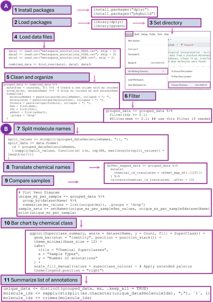
R‐script workflow for postprocessing METASPACE annotation. (A) Setup and data preparation: required R packages are installed and loaded, the working directory is set, METASPACE CSV files from multiple databases are imported and merged, and the combined table is cleaned/organized (m/z rounding, grouping by m/z × dataset, collapsing duplicate annotations) with optional filtering by FDR/MSM. (B) Downstream processing and reporting: multientry molecule‐name fields are parsed, chemical names are harmonized using RefMet, datasets are compared (e.g., overlap analyses), annotations are summarized by chemical class, and a refined, nonredundant annotation list is generated for subsequent targeted interpretation and visualization.

Table: Summary of libraries needed to use the script.

Examples of the Protocol Implementation

InExample S1, we compare sorghum stem sections from two developmental stages, 5‐ and 7‐week‐old (Figure5A). Annotation results with an FDR of 10% were processed using the described script. A Venn diagram (Figure5B) revealed 51 common features, 79 unique in the 5‐week sample, and 19 unique features in the 7‐week sample. The full list of unique and shared features, including superclass, class, and subclass information [27] can be found inFile S1.

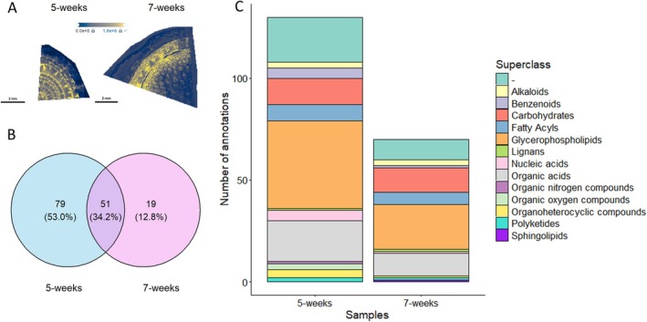
Comparison of MSI annotations between 5‐ and 7‐week sorghum stem samples. (A) Representative ion images for the same annotated feature shown in transverse stem sections at 5 and 7 weeks (scale bars indicate 2 mm; and intensity per the displayed color scale Cividis). (B) Venn diagram displays shared and sample‐specific annotatedm/zfeatures between the two datasets. (C) Superclass level classification of annotated features summarizing overall differences in the chemical composition between the samples.

Molecule names from the annotated list were harmonized to a standardized chemical nomenclature, and the resulting list of common names was used for chemical classification (Figure5C). In untargeted metabolomic experiments, such as MSI, this classification step is valuable because METASPACE annotations rely on molecular formulas, MSM scores, and FDRs [12]. Thus, organizing results into chemical categories provides an opportunity to begin exploring the biological context of the samples. For instance, changes in chemical classes can be determined and proportions of those under specific conditions can be visualized [34].

Figure5Cpresents a stacked bar plot comparing the number of annotated molecules classified into chemical superclasses based on the ChemOnt chemical taxonomy [27]. As is common in untargeted metabolomics, a significant proportion of molecules remain unclassified. This is largely because the Metabolomics Workbench does not provide standardized common names for all METASPACE annotations, leaving some classification fields blank in the output data frame. This is illustrated in Figure5Cwhere the first stacked bar (aqua color) represents unclassified features. Even without complete classification, differences in chemical superclass distribution between the two development stages are apparent. The younger stem sample contains higher number of organic acids and glycerophospholipids consistent with active metabolism, cell division, and cell expansion. By 7 weeks, these metabolites decrease, reflecting a development transition toward tissue maturation and reduced metabolic flux and lower membrane biosynthesis.

For the unclassified molecules, alternative strategies can improve name harmonization and further chemical classification. This step includes using a third‐party chemical translation tool that produces results similar to those in Figure4B‐8. Available tools include Classyfire, PubChem [35], the Human Metabolome Database (HMDB) [36], the LIPID MAPS, and the Chemical Translation Service (CTS) [37]. For users seeking deeper chemical classification, we recommend using CTS followed by the Batch Compound Classification (https://cfb.fiehnlab.ucdavis.edu/). FigureS1demonstrates this workflow.

InExample S2, we compare five kidney biopsy tissue sections representing different health conditions (Figure6A). Samples were interrogated in positive ion mode to measure lipids, and annotations were generated using the LIPID MAPS, SwissLipids, and HMDB databases. When focusing on lipids, the lipid enrichment tool within METASPACE can be applied; this tool is based on the Lipid Ontology (LION) enrichment analysis platform [38].

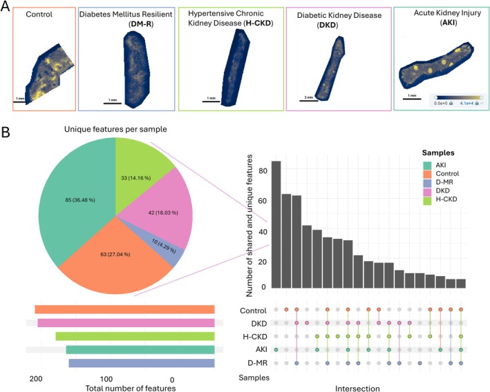
Cross‐sample comparison of MSI molecular annotations across kidney diseases. (A) MSI images of each sample type showing as an example them/z725.5568 corresponding to the molecular formula C39H79N2O6P and putatively annotated as C16 Sphingomyelin. Data are shown for control, diabetes mellitus–resilient (DM‐R), hypertensive chronic kidney disease (HCD‐K), diabetic kidney disease (DKD), and acute kidney injury (AKI) tissue. Total ion intensity normalization applied using the color scale Cividis. (B) Summary of ion features and their overlap across samples. The pie chart (left) reports the number (and percentage) of features that are unique to each sample type. The UpSet plot (right) summarizes the feature intersections: each vertical bar gives the number of features observed in the specific intersection indicated directly below by the connected filled dots (filled dot = feature present in that sample; gray dot = absent). Single‐dot columns therefore represent sample‐specific features, whereas multidot columns represent features shared by the connected set of samples only (e.g., pairs, triples, or higher order overlaps). Bars are ordered by intersection size (largest to smallest), allowing rapid identification of the shared feature sets across sample types.

In this example, we created an UpSet plot to compare the five samples to visualize the number of uniquem/zfeatures per sample, as well as the shared features among them (intersections).

Analysis of the UpSet plot (Figure6B) indicates that alongside the 32 commonm/zfeatures, each biopsy sample exhibits a distinct set of unique features. The AKI sample contained 85 unique features, compared with the 63 unique features in the control biopsy. These sample‐specific ions may reflect condition‐associated molecular differences and can serve as starting points for identifying candidate biomarkers.

To prioritize these molecular features, we applied an alternative analysis using the same R‐script. We focused specifically on unique features to each biopsy sample. Figure6B(pie chart) shows the proportion of unique features by each condition. As previously noted, the AKI sample comprises the highest proportion of unique features (36%), followed by the control samples (27%). FigureS2‐Bpresents the chemical classification of these unique features per sample, where sphingolipids are highly abundant in both AKI and DKD biopsies, likely because of their role in inflammation and mitochondrial dysfunction, the key points of tubular kidney injury [39].

All features in this example were harmonized and further classified, aided by an additional step of manual curation using online tools (FigureS1). Although time‐consuming, this step may be required when a complete classification is desired. The resulting UpSet plot data are available in the FileS2.

It is important to note that the chemical classifications presented here rely on the first molecule name listed in the combined METASPACE output. Therefore, we always recommend carefully reviewing the final dataset to identify potential inconsistencies or incorrect annotations. Although METASPACE provides accurate molecular formulas annotations [22], it does not differentiate between isomers. For this reason, themoleculeNamescolumn containing all putative identifications is retained in the final data file.

InExample S3, we present an example of a project submitted to METASPACE to showcase the broad applicability of the script, regardless of the ionization source employed in the experiment. In this published dataset [15], IR‐MALDI was systematically tested in positive ion mode using two solvent conditions, each with and without an ice matrix layer. The standard solvent consisted of 50:50 water:ACN with 0.2% formic acid, whereas the doped solvent included 70 μM NH4F. Mouse brain samples were analyzed under all four conditions, and the analyses targeted lipids. Data were uploaded to METASPACE and annotated using LIPID MAPS with a 10% FDR; full experimental details can be consulted in the original publication [15].

Figure7Ashows ion images, for an example feature with am/z369.3516 putatively annotated as 3‐Deoxyvitamin D3 and corroborated by the authors as cholesterol [M + H‐H2O]+. Figure7Bshows a four‐way Venn diagram illustrating the number of shared and unique features across the four experimental conditions. The doped solvent with an ice matrix produced the highest number of unique features (28.1%), followed by the standard solvent with ice (7.8%). These findings are consistent with the authors' observations as the use of an ice matrix is known to enhance molecular detection [40]. We did not evaluate ion intensities as it is in the original study. However, the total number of features with an ice matrix, supporting the reported enhancement (Figure7C). The corresponding data are provided in the FileS3. As expected, samples analyzed without an ice matrix yielded fewer annotated features, regardless of whether the dopant was included. Overall, this script provides an effective and rapid method for screening and summarizing METASPACE annotations. Additional analyses such as assessing relative abundances or spatial intensity patterns across tissue are not currently implemented and remain outside the scope of this workflow. However, because the code is open source, users are encouraged to adapt and extend it to meet their specific analytical needs.

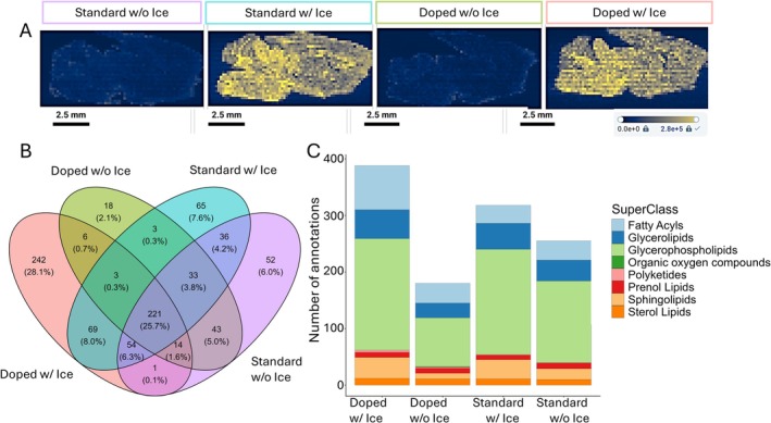
Comparison of METASPACE annotations across of MALDESI data using different sample/sampling‐preparation conditions. (A) Representative ion images for the same annotated feature withm/z369.3516 across four conditions: standard spray condition without ice, and with ice, NH4F‐doped solvent without ice, and with ice (total ion count normalization). (B) Four‐way Venn diagram summarizing overlapping of uniquem/zfeatures among conditions; numbers and percentages indicate features unique to each condition and shared across intersections. (C) Stacked bar plot showing the number of annotated features per chemical superclass for condition.

Conclusion

This protocol provides a user‐friendly R‐script that is particularly accessible for researchers new to MSI data analysis. The script offers clear advantages for untargeted MSI‐based spatial metabolomic experiments, especially when comparing different sample types or treatment groups. It enables a rapid overview of shared and unique annotations from METASPACE and organizes results for downstream biological interpretation through chemical classification. The R‐script is publicly available, and we encourage customization to expand and enhance its functionalities. Adding additional steps, libraries, and functions will further enhance the depth and flexibility of this initial MSI analysis workflow.

Conflicts of Interest

The authors declare no conflicts of interest.

References

1. H. Zhang, K. H. Lu, M. Ebbini, P. Huang, H. Lu, andL. Li, “Mass Spectrometry Imaging for Spatially Resolved Multi‐Omics Molecular Mapping, ”Npj Imaging2, no. 1(2024): 20, . From NLM PubMed‐not‐MEDLINE. doi.org/10.1038/s44303-024-00025-3
2. M. Stuwe, L. E. Petersen, andM. Liebeke, “From Microbes to Molecules: Unveiling Host‐Microbe Interactions With Spatial Metabolomics, ”Molecular Systems Biology21, no. 8(2025): 947–951, . From NLM In‐Process. doi.org/10.1038/s44320-025-00129-x
3. N. S. Garcia‐Rojas, C. D. Sierra‐Alvarez, H. E. Ramos‐Aboites, A. Moreno‐Pedraza, andR. Winkler, “Identification of Plant Compounds With Mass Spectrometry Imaging (MSI), ”Metabolites14, no. 8(2024): 491, From NLM PubMed‐not‐MEDLINE. doi.org/10.3390/metabo14080419
4. R. A. Shepherd, G. T. Luu, andL. M. Sanchez, “MALDI‐TIMS‐MS(2) Imaging and Annotation of Natural Products in Fungal‐Bacterial Coculture, ”Analytical Chemistry97, no. 35(2025): 18867–18872, From NLM Medline. doi.org/10.1021/acs.analchem.5c02787
5. B. L. Gorman, C. C. Shafer, N. Ragi, K. Sharma, E. K. Neumann, andC. R. Anderton, “Imaging and Spatially Resolved Mass Spectrometry Applications in Nephrology, ”Nature Reviews Nephrology21, no. 6(2025): 399–416, From NLM Medline. doi.org/10.1038/s41581-025-00946-1
6. A. R. Buchberger, K. DeLaney, J. Johnson, andL. Li, “Mass Spectrometry Imaging: A Review of Emerging Advancements and Future Insights, ”Analytical Chemistry90, no. 1(2018): 240–265. doi.org/10.1021/acs.analchem.7b04733
7. G. Baquer, L. Semente, T. Mahamdi, X. Correig, P. Rafols, andM. Garcia‐Altares, “What Are We Imaging? Software Tools and Experimental Strategies for Annotation and Identification of Small Molecules in Mass Spectrometry Imaging, ”Mass Spectrometry Reviews42, no. 5(2023): 1927–1964, From NLM PubMed‐not‐MEDLINE. doi.org/10.1002/mas.21794
8. T. Alexandrov, K. Ovchinnikova, A. Palmer, et al. , “METASPACE: A Community‐Populated Knowledge Base of Spatial Metabolomes in Health and Disease, ”bioRxiv1(2019): 539478, . doi.org/10.1101/539478
9. D. Velickovic, K. J. Zemaitis, A. Bhattacharjee, andC. R. Anderton, “Mass Spectrometry Imaging of Natural Carbonyl Products Directly From Agar‐Based Microbial Interactions Using 4‐APEBA Derivatization, ”mSystems9, no. 1(2024): e0080323, From NLM Medline. doi.org/10.1128/msystems.00803-23
10. D. Velickovic, T. Becejac, S. Mamedov, et al. , “Rapid Automated Annotation and Analysis of N‐Glycan Mass Spectrometry Imaging Data Sets Using NGlycDB in METASPACE, ”Analytical Chemistry93, no. 40(2021): 13421–13425, From NLM Medline. doi.org/10.1021/acs.analchem.1c02347
11. A. Rompp, T. Schramm, A. Hester, et al. , “imzML: Imaging Mass Spectrometry Markup Language: A Common Data Format for Mass Spectrometry Imaging, ”Methods in Molecular Biology696(2011): 205–224, From NLM Medline. doi.org/10.1007/978-1-60761-987-1_12
12. L. W. Sumner, A. Amberg, D. Barrett, et al. , “Proposed Minimum Reporting Standards for Chemical Analysis Chemical Analysis Working Group (CAWG) Metabolomics Standards Initiative (MSI), ”Metabolomics3, no. 3(2007): 211–221, . doi.org/10.1007/s11306-007-0082-2
13. J. R. Nunez, C. R. Anderton, andR. S. Renslow, “Optimizing Colormaps With Consideration for Color Vision Deficiency to Enable Accurate Interpretation of Scientific Data, ”PLoS ONE13, no. 7(2018): e0199239, From NLM Medline. doi.org/10.1371/journal.pone.0199239
14. B. Wadie, L. Stuart, C. M. Rath, B. Drotleff, S. Mamedov, andT. Alexandrov, “METASPACE‐ML: Context‐Specific Metabolite Annotation for Imaging Mass Spectrometry Using Machine Learning, ”Nature Communications15, no. 1(2024): 9110, From NLM Medline. doi.org/10.1038/s41467-024-52213-9
15. S. N. Hunter, M. F. Wang, B. N. Thomas, A. J. Filiano, andD. C. Muddiman, “Spatially Resolved Lipids in a Mouse Brain Model of Globoid Cell Leukodystrophy via IR‐MALDESI MSI and Parallel Reaction Monitoring MSI, ”Analytical and Bioanalytical Chemistry418, no. 7(2026): 1973–1986, From NLM Medline. doi.org/10.1007/s00216-026-06326-3
16. M. Kanehisa, M. Furumichi, M. Tanabe, Y. Sato, andK. Morishima, “KEGG: New Perspectives on Genomes, Pathways, Diseases and Drugs, ”Nucleic Acids Research45, no. D1(2017): D353–D361, From NLM Medline. doi.org/10.1093/nar/gkw1092
17. J. A. van Santen, G. Jacob, A. L. Singh, et al. , “The Natural Products Atlas: An Open Access Knowledge Base for Microbial Natural Products Discovery, ”ACS Central Science5, no. 11(2019): 1824–1833, . doi.org/10.1021/acscentsci.9b00806
18. M. Sud, E. Fahy, D. Cotter, et al. , “LMSD: LIPID MAPS Structure Database, ”Nucleic Acids Research35, no. Database Issue(2007): D527–D532, From NLM Medline. doi.org/10.1093/nar/gkl838
19. L. Aimo, R. Liechti, N. Hyka‐Nouspikel, et al. , “The SwissLipids Knowledgebase for Lipid Biology, ”Bioinformatics31, no. 17(2015): 2860–2866, From NLM Medline. doi.org/10.1093/bioinformatics/btv285
20. “R: A Language and Environment for Statistical Computing, ”2025, .
21. RStudio: Integrated Development Environment for R(Posit Software, 2025), .
22. A. Palmer, P. Phapale, I. Chernyavsky, et al. , “FDR‐Controlled Metabolite Annotation for High‐Resolution Imaging Mass Spectrometry, ”Nature Methods14, no. 1(2017): 57–60, . doi.org/10.1038/nmeth.4072
23. K. Ovchinnikova, V. Kovalev, L. Stuart, andT. Alexandrov, “OffsampleAI: Artificial Intelligence Approach to Recognize Off‐Sample Mass Spectrometry Images, ”BMC Bioinformatics21, no. 1(2020): 129, From NLM Medline. doi.org/10.1186/s12859-020-3425-x
24. S. M. Eisenberg, K. T. Knizner, andD. C. Muddiman, “Development of an Object‐Based Image Analysis Tool for Mass Spectrometry Imaging Ion Classification, ”Analytical and Bioanalytical Chemistry415, no. 19(2023): 4725–4730, From NLM Medline. doi.org/10.1007/s00216-023-04764-x
25. E. FahyandS. Subramaniam, “RefMet: A Reference Nomenclature for Metabolomics, ”Nature Methods17, no. 12(2020): 1173–1174, From NLM Medline. doi.org/10.1038/s41592-020-01009-y
26. The Metabolomics Workbench, .
27. Y. Djoumbou Feunang, R. Eisner, C. Knox, et al. , “ClassyFire: Automated Chemical Classification With a Comprehensive, Computable Taxonomy, ”Journal of Cheminformatics8(2016): 61, . doi.org/10.1186/s13321-016-0174-y
28. E. Fahy, M. Sud, D. Cotter, andS. Subramaniam, “LIPID MAPS Online Tools for Lipid Research, ”Nucleic Acids Research35, no. Web Server issue(2007): W606–W612, From NLM Medline. doi.org/10.1093/nar/gkm324
29. J. R. Conway, A. Lex, andN. Gehlenborg, “UpSetR: An R Package for the Visualization of Intersecting Sets and Their Properties, ”Bioinformatics33, no. 18(2017): 2938–2940, From NLM Medline. doi.org/10.1093/bioinformatics/btx364
30. G. Robichaud, K. P. Garrard, J. A. Barry, andD. C. Muddiman, “MSiReader: An Open‐Source Interface to View and Analyze High Resolving Power MS Imaging Files on Matlab Platform, ”Journal of the American Society for Mass Spectrometry24, no. 5(2013): 718–721, From NLM Medline. doi.org/10.1007/s13361-013-0607-z
31. S. Gibb, “MALDIquant, “ (2011), . doi.org/10.32614/CRAN.package
32. K. D. Bemis, A. Harry, L. S. Eberlin, et al. , “Cardinal: An R Package for Statistical Analysis of Mass Spectrometry‐Based Imaging Experiments, ”Bioinformatics (Oxford, England)31, no. 14(2015): 2418–2420, From NLM Medline. doi.org/10.1093/bioinformatics/btv146
33. I. Rosas‐Román, C. Ovando‐Vázquez, A. Moreno‐Pedraza, H. Guillén‐Alonso, andR. Winkler, “Open LabBot and RmsiGUI: Community Development Kit for Sampling Automation and Ambient Imaging, ”Microchemical Journal152(2020): 152, . doi.org/10.1016/j.microc.2019.104343
34. G. Hajjar, M. C. Barros Santos, J. Bertrand‐Michel, et al. , “Scaling‐Up Metabolomics: Current State and Perspectives, ”TrAC Trends in Analytical Chemistry167(2023): 167, . doi.org/10.1016/j.trac.2023.117225
35. S. Kim, P. A. Thiessen, E. E. Bolton, et al. , “PubChem Substance and Compound Databases, ”Nucleic Acids Research44, no. D1(2016): D1202–D1213, From NLM Medline. doi.org/10.1093/nar/gkv951
36. D. S. Wishart, Y. D. Feunang, A. Marcu, et al. , “HMDB 4. 0: The Human Metabolome Database for 2018, ”Nucleic Acids Research46, no. D1(2018): D608–D617, . doi.org/10.1093/nar/gkx1089
37. CTS ‐ The Chemical Translation Service, .
38. M. R. Molenaar, A. Jeucken, T. A. Wassenaar, C. H. A. van de Lest, J. F. Brouwers, andJ. B. Helms, “LION/Web: A Web‐Based Ontology Enrichment Tool for Lipidomic Data Analysis, ”GigaScience8, no. 6(2019): giz061, From NLM Medline. doi.org/10.1093/gigascience/giz061
39. Y. Wang, L. Wu, X. Bao, et al. , “Lipid Metabolic Dysregulation in Diabetic Kidney Disease: Mechanisms, Cellular Impact, and Therapeutic Strategies, ”Journal of Clinical & Translational Endocrinology44(2026): 100436, . doi.org/10.1016/j.jcte.2026.100436
40. G. Robichaud, J. A. Barry, andD. C. Muddiman, “IR‐MALDESI Mass Spectrometry Imaging of Biological Tissue Sections Using Ice as a Matrix, ”Journal of the American Society for Mass Spectrometry25, no. 3(2014): 319–328, From NLM Medline. doi.org/10.1007/s13361-013-0787-6

---

Republished from the open web under CC-BY. Authors: Moreno-Pedraza A, Gorman B, Velickovic M, Bentelspacher M, Barros J, Velickovic D, Anderton CR. Read the original.