Dipolar Order Mapping Based on Spin-Lock Magnetic Resonance Imaging.

Introduction

In ordered tissues containing motion‐restricted macromolecules, such as myelin, dipolar order exists alongside Zeeman order. This phenomenon manifests in magnetization transfer (MT) experiments as an asymmetric spectrum following single‐frequency saturation, in contrast to the symmetric spectrum observed under dual‐frequency saturation. Known as inhomogeneous magnetization transfer (ihMT), this effect can be quantified by the dipolar relaxation time,$T_{1 D}$, and is highly sensitive to tissue microstructure [1,2,3,4,5]. Consequently, ihMT offers a promising approach for assessing microstructural integrity, particularly brain myelination [6,7]. It holds significant potential for elucidating disease pathophysiology (e.g., in multiple sclerosis) and providing valuable outcome measures to monitor neuroprotection and repair in clinical trials [8,9,10].

The two‐pool model is commonly used to analyze the MT effect, while Provotorov theory, as formulated by Goldman for the dipolar order effect [1], indicates that the MT pool can be subdivided into a Zeeman reservoir and a dipolar reservoir. The parameter$\beta$, proportional to the inverse spin temperature of the dipolar reservoir, is incorporated into the two‐pool model [2,3,11]. To measure dipolar order under in vivo conditions, Varma et al. introduced ihMT ratio (ihMTR) for in vivo experiments to indicate the ihMT effect via a subtraction experiment between images acquired with single frequency saturation and dual frequency saturation [4]. They further proposed$T_{1 D}$quantification using multiple ihMTR images with varied switch times during dual‐frequency saturation [6]. However, this approach requires a long scan time to acquire sufficient ihMTR images (e.g., eight ihMTR images with different switch times [6]). Prevost et al. proposed an optimized ihMT acquisition strategy based on$T_{1 D}$filtering effect [12], which enables the isolation of short‐ and long‐$T_{1 D}$components by manipulating switch times [13]. Hertanu et al. further showed that the long‐$T_{1 D}$component is highly specific to myelination, whereas short‐$T_{1 D}$components are associated with nonmyelin protons [14]. These findings indicate that multiple ihMTR measurements are needed when the objective is to resolve multiple dipolar components with distinct$T_{1 D}$values. By contrast, under the simplifying assumption of an apparent single long‐$T_{1 D}$component and fixed MT parameters, a single or limited number of ihMT measurements may be sufficient for$T_{1 D}$estimation.

In parallel, a pseudo‐quantitative ihMT method based on inverse‐subtraction metrics has also been developed [9,15]. This approach enables rapid acquisition with good reproducibility and reduced sensitivity to several confounding factors, and it has been applied in human studies [16,17,18]. Malik et al. further proposed a rapid steady‐state pulse sequence for generating ihMT contrast using multiband RF pulses, which simultaneously provide off‐resonance saturation and on‐resonance excitation [19]. Nevertheless, these approaches remain semiquantitative and do not directly quantify dipolar order. More recently, West et al. proposed an MR fingerprinting framework for quantifying$T_{1 D}$, macromolecular proton fraction (MPF), and the$T_{1}$of the free‐water pool [20]. Despite these advances, the development of methods for$T_{1 D}$quantification that can assess myelin microstructural integrity while minimizing confounding effects and maintaining clinically feasible scan times remains highly valuable [8,21,22].

Recently, an off‐resonance spin‐lock approach (MPF‐SL) was proposed for quantitative MT [23,24,25]. In MPF‐SL, appropriately designed off‐resonance spin‐lock acquisitions are used to remove the free‐water contribution from the rotating‐frame relaxation rate,$R_{1 \rho}$. This yields an MT‐specific relaxation rate,$R_{\textit{mpfsl}}$, from which MPF can be estimated. Consequently, MPF‐SL allows the use of RF pulses with higher saturation efficiency without exacerbating direct water saturation. By isolating the macromolecular contribution from the water‐pool contribution, this approach substantially simplifies the model for MPF quantification and eliminates the need for prior knowledge or separate estimation of free‐water relaxation times. In addition, the off‐resonance spin‐lock design enables this method to suppress residual dipolar coupling effects in clinical scans [26,27].

In this study, we extend this approach to quantify the dipolar relaxation time,$T_{1 D}$, under the assumption of a single apparent long‐$T_{1 D}$component. With our proposed method, both the MPF and$T_{1 D}$can be acquired in a single fast scan, providing complementary information for tissue assessment. To probe the ihMT effect, we utilize a chain of rotary echo spin‐lock radiofrequency (RF) pulses with variable switch times. These pulses alternate between positive and negative resonance frequency offsets, synchronized with RF phase alterations, to maintain magnetization spin‐locking throughout the pulse duration. These spin‐lock acquisitions eliminate free water contributions from the signal model, thereby substantially simplifying the calculation of$T_{1 D}$. Furthermore, MPF is quantified from the same dataset without requiring additional scans. We demonstrate the efficacy of this method using numerical simulations, phantom experiments, and in vivo measurements.

Theory

In the two‐pool model for MT, tissue magnetization is commonly divided into a water pool ($M_{x}^{a} , M_{y}^{a} , \text{and} M_{z}^{a}$) and an MT pool ($M_{z}^{b}$) [28]. Based on Provotorov theory as formulated by Goldman [1], the MT pool can be further described as comprising both a Zeeman reservoir and a dipolar reservoir. The parameter$\beta$, which is proportional to the inverse spin temperature of the dipolar reservoir, is incorporated into the magnetization vector [2,3,11]

$$\overset{\rightarrow}{M} = \left(\left(M_{\mathit{ax}},M_{\mathit{ay}},M_{\mathit{az}},M_{\mathit{bz}},\beta\right)\right)^{T} ,$$

which follows:

$$\frac{d}{\mathit{dt}} \overset{\rightarrow}{M} = A \cdot \overset{\rightarrow}{M} + \overset{\rightarrow}{C} .$$

Following the notation by Zaiss et al. [29] and incorporating dipolar order [11], we express$A$as a 5 × 5 system matrix:

$$\begin{matrix}\begin{matrix}A = \begin{pmatrix} \begin{matrix}- R_{2 a} & - Δω & 0 & 0 & 0 \\ + Δω & - R_{2 a} & + \omega_{1} & 0 & 0 \\ 0 & - \omega_{1} & - R_{1 a} - k_{\mathit{ab}} & k_{\mathit{ba}} & 0 \\ 0 & 0 & k_{\mathit{ab}} & - R_{1 b} - R_{\mathit{rfb}} - k_{\mathit{ba}} & R_{\mathit{rfb}} \Delta \omega \\ 0 & 0 & 0 & R_{\mathit{rfb}} \frac{\Delta \omega}{D^{2}} & - \left(\frac{1}{T_{1 D}} + R_{\mathit{rfb}} \left(\frac{\Delta \omega}{D}\right)^{2}\right)\end{matrix} \end{pmatrix}\end{matrix}\end{matrix}$$

and$\overset{\rightarrow}{C}$is a constant vector:

$$\overset{\rightarrow}{C} = \left(0 , 0 , R_{1 a} M_{0 a} , R_{1 b} M_{0 b} , 0\right)^{T}$$

where$T_{1 D}$is the dipolar relaxation time.$R_{2 a}$and$R_{1 a}$are the transverse and longitudinal relaxation rates for the water pool, respectively.$R_{1 b}$is the longitudinal relaxation rate for the MT pool.$R_{\mathit{rfb}} = \omega_{1}^{2} \mathit{πg} \left(T_{2 b},\Delta \omega\right)$, where$g \left(T_{2 b},\Delta \omega\right)$denotes the absorption lineshape of the MT pool, and we use a super‐Lorentzian lineshape model in this study [3].$T_{2 b}$is an MT‐pool parameter that characterizes its absorption lineshape.$M_{0 a}$and$M_{0 b}$denote the equilibrium magnetizations of the water and MT pools, respectively.$\Delta \omega$is the resonance frequency offset (FO) and$\omega_{1}$is the$B_{1}$amplitude of the spin‐lock RF pulse, or equivalently the frequency of spin‐lock (FSL).$k_{\mathit{ab}}$and$k_{\mathit{ba}}$are the exchange rates between the water pool and the MT pool. D is associated with the local dipolar field (in angular frequency units) [3], which approximately equals to$\frac{1}{T_{2 b} \sqrt{15}}$. In addition, we assume the fraction of dipolar order$f_{D}$= 1 [3,11].

When dual‐frequency RF is applied with simultaneous irradiation at positive and negative frequency offsets, the term proportional to$\Delta \omega$in Equation3is canceled. It indicates the contribution from dipolar reservoir can be removed using dual‐frequency RF irradiation. Consequently,$A_{\textit{dual}}$simplifies to:

$$A_{\textit{dual}} = \begin{pmatrix} - R_{2 a} & - \mathit{Δω} & 0 & 0 \\ + \mathit{Δω} & - R_{2 a} & + \omega_{1} & 0 \\ 0 & - \omega_{1} & - R_{1 a} - k_{\mathit{ab}} & + k_{\mathit{ba}} \\ 0 & 0 & + k_{\mathit{ab}} & - R_{1 b} - R_{\mathit{rf} b} - k_{\mathit{ba}} \end{pmatrix}$$

In the rotating frame, the relaxation rates$R_{1 \rho}$measured under single‐frequency spin‐lock irradiation ($R_{1 \rho}^{\text{single}}$, with$\Delta \omega^{s}$and$\omega_{1}^{s}$) and dual‐frequency spin‐lock irradiation ($R_{1 \rho}^{\text{dual}}$, with$\Delta \omega^{d}$and$\omega_{1}^{d}$) are primarily determined by the least negative eigenvalue of$A$and$A_{\textit{dual}}$[29,30], respectively:

$$R_{1 \rho}^{\textit{single}} = R_{W} \left(\mathit{Δω}^{s},\left(\omega_{1}\right)^{s}\right) + R_{\mathit{MT}}^{s} \left(\mathit{Δω}^{s},\left(\omega_{1}\right)^{s}\right)$$

and

$$R_{1 \rho}^{\textit{dual}} = R_{W} \left(\mathit{Δω}^{d},\left(\omega_{1}\right)^{d}\right) + R_{\mathit{MT}}^{d} \left(\mathit{Δω}^{d},\left(\omega_{1}\right)^{d}\right)$$

Here,$R_{W}$represents the effective relaxation rate of the water pool, whereas$R_{\mathit{MT}}^{s}$and$R_{\mathit{MT}}^{d}$denote the relaxation rates associated with the MT pool under single‐frequency and dual‐frequency spin‐lock irradiation, respectively. Notably,$R_{1 \rho}^{\textit{single}}$contains a contribution from dipolar order, whereas this contribution is suppressed in$R_{1 \rho}^{\text{dual}}$. Under the conditions$\mathit{Δω}^{d} \gg \left(\omega_{1}\right)^{d}$and$\mathit{Δω}^{s} \gg \left(\omega_{1}\right)^{s}$, the influence of chemical exchange is negligible. When single‐frequency and dual‐frequency spin‐lock are applied with the same direction of spin‐lock field (i.e.,$\frac{\Delta \omega^{d}}{\omega_{1}^{d}} = \frac{\Delta \omega^{s}}{\omega_{1}^{s}}$), the water pool contribution$R_{W}$can be removed by taking the difference between$R_{1 \rho}^{\textit{single}}$and$R_{1 \rho}^{\textit{dual}}$. We therefore define a distinct relaxation rate,$R_{\textit{dosl}}$, associated with the ihMT effect (seeSupporting Information 1for details):

$$\begin{matrix}\begin{matrix}R_{\textit{dosl}} = R_{1 \rho}^{\textit{dual}} - R_{1 \rho}^{\textit{single}} = R_{\mathit{MT}}^{d} - R_{\mathit{MT}}^{s} \\ = f_{b} k_{\mathit{ba}} \left[\frac{R_{\mathit{rfb}}^{d}}{k_{\mathit{ba}} \left(f_{b} + 1\right) + R_{\mathit{rfb}}^{d}} - \frac{R_{\mathit{rfb}}^{s}}{k_{\mathit{ba}} \left(f_{b} + 1\right) \left(R_{\mathit{rfb}}^{s} \left(\frac{\Delta \omega^{s}}{D}\right)^{2} T_{1 D} + 1\right) + R_{\mathit{rfb}}^{s}}\right]\end{matrix}\end{matrix}$$

Here,$R_{\mathit{rfb}}^{s}$and$R_{\mathit{rfb}}^{d}$correspond to the absorption lineshape terms under single‐frequency and dual‐frequency spin‐lock conditions, respectively. By definition,$k_{\mathit{ba}} = R \left(1 - f_{b}\right)$, where$R$is the exchange rate. Because$f_{b}$typically ranges from 0.11 to 0.15 in human white matter [31], implying$f_{b}^{2} \ll 1$, we have$k_{\mathit{ba}} \left(f_{b} + 1\right) = R \left(1 - f_{b}^{2}\right) \approx R$. Accordingly, Equation (8) can be simplified to:

$$\begin{matrix}R_{\textit{dosl}} = R_{1 \rho}^{\textit{dual}} - R_{1 \rho}^{\textit{single}} = R_{\mathit{MT}}^{d} - R_{\mathit{MT}}^{s} \\ = f_{b} R \left(1 - f_{b}\right) \left[\frac{R_{\mathit{rfb}}^{d}}{R + R_{\mathit{rfb}}^{d}} - \frac{R_{\mathit{rfb}}^{s}}{R \left(R_{\mathit{rfb}}^{s} \left(\frac{\Delta \omega^{s}}{D}\right)^{2} T_{1 D} + 1\right) + R_{\mathit{rfb}}^{s}}\right]\end{matrix}$$

To further improve the robustness of$T_{1 D}$estimation, we introduce a variable,$\textit{RATIO}_{\textit{dosl}}$, defined as the ratio of$R_{\textit{dosl}}$measured under two different spin‐lock conditions, denoted$R_{\textit{dosl} , 1}$and$R_{\textit{dosl} , 2}$, with distinct combinations of$Δω$and$\omega_{1}$. We impose the following conditions, satisfied in both theoretical derivation and practical implementation:

$$\frac{\Delta \omega^{d \left(1\right)}}{\omega_{1}^{d \left(1\right)}} = \frac{\Delta \omega^{d \left(2\right)}}{\omega_{1}^{d \left(2\right)}} = \frac{\Delta \omega^{s \left(1\right)}}{\omega_{1}^{s \left(1\right)}} > > 1 ,$$ $$\Delta \omega^{d \left(1\right)} = \Delta \omega^{s \left(1\right)} ,$$

and

$$\frac{\omega_{1}^{d \left(1\right)}}{\omega_{1}^{d \left(2\right)}} = \frac{\Delta \omega^{d \left(1\right)}}{\Delta \omega^{d \left(2\right)}} = N \left(N > 1\right) .$$

Under these conditions,$\textit{RATIO}_{\textit{dosl}}$is given by:

$$\begin{matrix}\textit{RATIO}_{\textit{dosl}} = \frac{R_{\textit{dosl} , 1}}{R_{\textit{dosl} , 2}} = \frac{R_{1 \rho}^{\textit{dual} \left(1\right)} - R_{1 \rho}^{\textit{single} \left(1\right)}}{R_{1 \rho}^{\textit{dual} \left(2\right)} - R_{1 \rho}^{\textit{single} \left(1\right)}} \\ = \left[\frac{R + R_{\mathit{rfb}}^{d \left(2\right)}}{R + R_{\mathit{rfb}}^{d \left(1\right)}} \star \frac{R_{\mathit{rfb}}^{d \left(1\right)} R_{\mathit{rfb}}^{s \left(1\right)} \left(\frac{\Delta \omega^{s \left(1\right)}}{D}\right)^{2} T_{1 D}}{R_{\mathit{rfb}}^{d \left(2\right)} \left(R_{\mathit{rfb}}^{s \left(1\right)} \left(\frac{\Delta \omega^{s \left(1\right)}}{D}\right)^{2} T_{1 D} + 1\right) - R_{\mathit{rfb}}^{s \left(1\right)}}\right]\end{matrix}$$

In quantitative MT, the exchange rate$R$and the lineshape parameter$T_{2 b}$are often treated as constants in human studies [32]. Under this assumption,$\textit{RATIO}_{\textit{dosl}}$is primarily associated with the dipolar relaxation time$T_{1 D}$, allowing$T_{1 D}$to be estimated conveniently from$\textit{RATIO}_{\textit{dosl}}$. Notably, MPF can be calculated from$R_{1 \rho}^{\text{dual} \left(1\right)}$and$R_{1 \rho}^{\text{dual} \left(2\right)}$following the method of Hou et al. [23]. This approach removes the confounding influence of dipolar order on MPF estimation without requiring additional data acquisition.

Method

Acquisition Scheme

In existing ihMT acquisition schemes, dual‐frequency saturation can be applied using rapid alternation at positive and negative frequency offsets on a minimal timescale [6]. Similarly, we propose using a chain of rotary echo spin‐lock RF pulses to probe the ihMT effect. In this implementation, the spin‐lock RF pulses alternate between positive and negative resonance frequency offsets with a switching time,$T_{s}$. To maintain magnetization spin‐locking throughout the pulse duration, the RF phase is alternated in synchronization with the frequency offsets. Owing to the$T_{1 D}$filtering effect [13,14], dual‐frequency spin‐lock is achieved when$T_{s}$is shorter than the tissue$T_{1 D}$(Figure1a). In contrast, single‐frequency spin‐lock is implemented using a long$T_{s}$that considerably exceeds the tissue$T_{1 D}$(Figure1b). This modified rotary‐echo spin‐lock RF pulse sequence therefore provides a practical method to acquire$R_{1 \rho}^{\textit{single}}$and$R_{1 \rho}^{\textit{dual}}$.

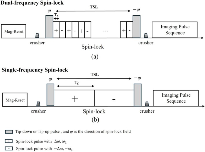
(a) Dual‐frequency spin‐lock pulse sequence with a short switch timeTs(shorter than the tissueT1D). (b) Single‐frequency spin‐lock pulse sequence with a long switch timeTs(longer than the tissueT1D).

For in vivo experiments, direct measurement of$R_{1 \rho}^{\textit{single}}$and$R_{1 \rho}^{\textit{dual}}$can be challenging. Robust quantification requires multiple spin‐lock‐prepared images acquired over sufficiently long spin‐lock times (TSLs), which is constrained by specific absorption rate (SAR) and RF hardware limitations. Following the approach reported by Hou et al. [23,33], we instead acquire data that allow direct calculation of the difference of$R_{1 \rho}^{\textit{single}}$and$R_{1 \rho}^{\textit{dual}}$, rather than measuring the two rates individually. Specifically,$R_{\textit{dosl}} = R_{1 \rho}^{\textit{dual}} - R_{1 \rho}^{\textit{single}}$can be obtained from two spin‐lock prepared images using the fast acquisition strategy described by Hou et al. [33]. Consequently,$\textit{RATIO}_{\textit{dosl}}$can be calculated using a total of only three spin‐lock prepared images:

$$\begin{matrix}\textit{RATIO}_{\textit{dosl}} = \frac{R_{\textit{dosl} , 1}}{R_{\textit{dosl} , 2}} = \frac{R_{1 \rho}^{\textit{dual} \left(1\right)} - R_{1 \rho}^{\textit{single} \left(1\right)}}{R_{1 \rho}^{\textit{dual} \left(2\right)} - R_{1 \rho}^{\textit{single} \left(1\right)}} \\ = \frac{- log \left(\frac{M_{d}^{\left(1\right)} - M_{d , \mathit{ini}}^{\left(1\right)}}{M_{s}^{\left(1\right)} - M_{s , \mathit{ini}}^{\left(1\right)}}\right) / \mathit{TSL}}{- log \left(\frac{M_{d}^{\left(2\right)} - M_{d , \mathit{ini}}^{\left(2\right)}}{M_{s}^{\left(1\right)} - M_{s , \mathit{ini}}^{\left(1\right)}}\right) / \mathit{TSL}} \\ \approx \frac{- log \left(\frac{M_{d}^{\left(1\right)}}{M_{s}^{\left(1\right)}}\right) / \mathit{TSL}}{- log \left(\frac{M_{d}^{\left(2\right)}}{M_{s}^{\left(1\right)}}\right) / \mathit{TSL}}\end{matrix}$$

Here,$M_{d}^{\left(1\right)}$and$M_{d}^{\left(2\right)}$denote the dual‐frequency spin‐lock prepared images corresponding to relaxation rates$R_{1 \rho}^{\textit{dual} \left(1\right)}$and$R_{1 \rho}^{\textit{dual} \left(2\right)}$, respectively.$M_{s}^{\left(1\right)}$denotes the single‐frequency spin‐lock prepared image associated with$R_{1 \rho}^{\textit{single} \left(1\right)}$. The subscript “ini” denotes spin‐lock‐prepared images acquired with a different initial magnetization, which are used to remove the influence of steady‐state magnetization [23]. In brain applications, acquisition of these images can be omitted according to the theory described in the fast acquisition strategy of Hou et al. [33].

Calculation ofT1D

The workflow for calculating$T_{1 D}$consists of two steps, as illustrated in Figure2. In the first step,$\textit{RATIO}_{\textit{dosl}}$is computed from$R_{\textit{dosl} , 1}$and$R_{\textit{dosl} , 2}$using three off‐resonance spin‐lock prepared images according to Equation11. In the second step, the$T_{1 D}$map is estimated from$\textit{RATIO}_{\textit{dosl}}$. While multiple numerical approaches exist for this estimation, this study investigates both an analytical estimation and a dictionary‐matching approach. The analytical estimation determines$T_{1 D}$directly by solving Equation10using experimentally observed$\textit{RATIO}_{\textit{dosl}}^{\mathit{acq}}$. In contrast, the dictionary‐matching approach generates a$\textit{RATIO}_{\textit{dosl}}$dictionary over a predefined range of$T_{1 D}$values;$T_{1 D}$is then determined by matching the measured$\textit{RATIO}_{\textit{dosl}}$to the corresponding entry in the dictionary.

Workflow of theT1Dcalculation. In Step 1,RATIOdoslis calculated from three spin‐lock prepared images,Ms1,Md1, andMd2. In Step 2,T1Dis derived from theRATIOdoslvalues. An MPF map can be obtained fromMd1andMd2in an optional step [23].

Under fixed spin‐lock pulse settings and tissue parameters of the two‐pool model,$\textit{RATIO}_{\textit{dosl}}$is a one‐to‐one function of$T_{1 D}$. Accordingly, for each candidate$T_{1 D}$, three magnetizations ($M_{d}^{\left(1\right)}$,$M_{d}^{\left(2\right)}$and$M_{s}^{\left(1\right)}$) are simulated using Bloch‐McConnell‐Provotorov equation (Equation1–5) following the modified rotary‐echo spin‐lock RF pulses (Figure1), and the corresponding$\textit{RATIO}_{\textit{dosl}}$is then derived via Equation11. The spin‐lock parameters are fixed to match the practical MRI acquisition setup, and tissue parameters of the water pool and the MT pool are held constant according to literature or preacquisition measurements (see Section3.4.3for details).

Note the amplitude of RF pulse is incorporated into the lineshape function$R_{\mathit{rfb}}$. Consequently, to calculate$T_{1 D}$from$\textit{RATIO}_{\textit{dosl}}$, a$B_{1}$map is acquired to convert the nominal spin‐lock RF amplitude into the actual applied RF amplitude. Given the measured$\textit{RATIO}_{\textit{dosl}}^{\mathit{acq}}$and the corresponding local$B_{1}$value, the optimal entry in the dictionary is identified by minimizing the residual between$\textit{RATIO}_{\textit{dosl}}^{\mathit{acq}}$and the simulated$\textit{RATID}_{\textit{dosl}}$. The$T_{1 D}$value associated with this best match is then assigned as the estimated$T_{1 D}$.

Simulation Studies

The simulation studies were conducted to validate the proposed theory and the acquisition approach. In all simulation studies, the designed conditions for spin‐lock acquisition parameters were set as:$\frac{\Delta \omega^{d \left(1\right)}}{\omega_{1}^{d \left(1\right)}} = \frac{\Delta \omega^{d \left(2\right)}}{\omega_{1}^{d \left(2\right)}} = \frac{\Delta \omega^{s \left(1\right)}}{\omega_{1}^{s \left(1\right)}}$=10,$\Delta \omega^{d \left(1\right)} = \Delta \omega^{s \left(1\right)}$, and$\frac{\omega_{1}^{d \left(1\right)}}{\omega_{1}^{d \left(2\right)}} = \frac{\Delta \omega^{d \left(1\right)}}{\Delta \omega^{d \left(2\right)}} = 5$. In Simulation study 1, to enable a comprehensive analysis, we vary$\Delta \omega^{d \left(1\right)}$and$\omega_{1}^{d \left(1\right)}$, and the remaining parameters are adjusted accordingly to satisfy these design conditions. All simulations were performed using custom MATLAB code, which is available on GitHub (https://github.com/zjgao‐spin/Dipolar‐order‐mapping).

Simulation Study 1: Accuracy of Quantification

Accuracy of ApproximatedRADIOdosl

To assess the accuracy of this analytical expression of$\textit{RATIO}_{\textit{dosl}}$at Equation10, we compared it against the exact numerical solution of$\textit{RATIO}_{\textit{dosl}}$obtained by integrating the Bloch‐McConnell‐Provotorov equations. For this comparison, we utilized tissue parameters for white matter derived from previous publications [34,35]:$T_{1 a} = 1840 \mathit{ms}$,$T_{1 b} = 340 \mathit{ms}$,$T_{2 a} = 69 \mathit{ms}$,$T_{2 b} = 10 \mathit{μs}$,$\mathit{MPF} = 15 \%$, and$R = 23 s^{- 1}$. We evaluated$T_{1 D}$values of 2, 4, 6, and 8 ms, consistent with the previously reported range for white matter [6,14]. The ranges for$\mathit{Δω}^{d \left(1\right)}$and$\omega_{1}^{d \left(1\right)}$were set to cover common experimental values: 2–7 kHz and 200–800 Hz, respectively. Furthermore, to theoretically validate the sensitivity of the method, we analyzed the relationship between$\textit{RATIO}_{\textit{dosl}}$and$T_{1 D}$across a range of 1 to 10 ms. Additionally, we investigated how$\textit{RATIO}_{\textit{dosl}}$varies with other tissue parameters, including$R_{1 a}$(0.3–1.5 Hz),$R_{2 a}$(10–70 Hz),$R_{1 b}$(2–5 Hz),$R$(15–25 Hz),$\mathit{MPF}$(10%–20%), and$T_{2 b}$(9–11 μs).

Accuracy ofT1DQuantification

The analytical estimation does not require generating a dictionary. However, when using this method, the approximate$\textit{RATIO}_{\textit{dosl}}$model (Equation10) can introduce bias in the estimated$T_{1 D}$due to underlying theoretical assumptions. This bias between the estimated and ground‐truth$T_{1 D}$can be mitigated by the appropriate selection of acquisition parameters.

To identify parameter regimes that minimize the bias when using the approximate model, we computed the error in the estimated$T_{1 D}$relative to a ground‐truth value of$T_{1 D}$= 6.2 ms [6]. Acquired$\textit{RATIO}_{\textit{dosl}}$values were generated via numerical simulations using Equations1–5and11. The switch times,$T_{s}$, for the dual and single‐frequency spin‐lock pulses were chosen as 0.5 and 40 ms, respectively, given that white matter$T_{1 D}$typically ranges from 3 to 10 ms [7]. The simulation parameters were set as follows:$\Delta \omega^{d \left(1\right)} / 2 \pi$from 2 to 7 kHz,$\omega_{1}^{d \left(1\right)} / 2 \pi$ranged from 200 to 800 Hz, TSL from 40 to 120 ms$.$The$T_{1 D}$values were then calculated by solving Equation10.

Simulation Study 2: Robustness of the Proposed Method

Robustness in Presence of B1 and B0 Inhomogeneity

$B_{1}$and$B_{0}$field inhomogeneities are common in MRI systems. We performed simulations to investigate the robustness of the proposed method in the presence of these inhomogeneities. The simulations utilized the same spin‐lock pulse and tissue parameters for white matter as those used in Simulation Study 1, with$\Delta \omega^{d \left(1\right)} / 2 \pi$,$\omega_{1}^{d \left(1\right)} / 2 \pi$and TSL fixed at 5 kHz, 500 Hz and 80 ms, respectively.$B_{1}$and$B_{0}$were varied over ranges of 0.7 to 1.3 n.u. and −100 to 100 Hz, respectively.$B_{1}$and$B_{0}$inhomogeneities were incorporated throughout the entire spin‐lock preparation, including the tip‐down, spin‐lock, and tip‐up pulses. Note the flip angle used for the tip‐down and tip‐up pulses was$\mathit{tan}^{- 1} \left(\omega_{1} / \Delta \omega\right)$.

Furthermore, we compared the mean and standard deviation of the estimated$T_{1 D}$with and without$B_{1}$inhomogeneity correction. In this analysis,$B_{1}$and$B_{0}$values were sampled 10,000 times from a uniform distribution over respective range.$T_{1 D}$was estimated using both analytical estimation and dictionary matching. The dictionary was generated covering a$B_{1}$range of 0.7–1.3 (step size$1 \times 10^{- 4}$) and a$T_{1 D}$range of 0–15 ms (step size$1 \times 10^{- 5}$ms).

Robustness Against Variations of the Tissue Parameters

Like other quantitative MT methods, we assumed that certain MT parameters remain constant when calculating$T_{1 D}$.$\textit{RATIO}_{\textit{dosl}}$is predicted to have low sensitivity to most MT parameters, except for$T_{2 b}$. In this study, we performed simulations to investigate the errors in the estimation of$T_{1 D}$when MT parameters, specifically$R_{1 b}$,$R$, and MPF, are not constant. We conducted 10,000 simulations with parameters randomly sampled within the following ranges:$R_{1 b} = 2$–5 Hz,$R$= 15–25 Hz, and MPF = 10%–20%. We then calculated the variation of the estimated$T_{1 D}$under these parameter variations.

Robustness Against Noise

Quantitative imaging requires a sufficient signal‐to‐noise ratio (SNR). In this study, we investigated the influence of SNR on$\textit{RATIO}_{\textit{dosl}}$and$T_{1 D}$estimation. Simulated MRI signals$M_{d}^{\left(1\right)}$,$M_{d}^{\left(2\right)}$, and$M_{s}^{\left(1\right)}$were corrupted with additive white Gaussian noise at SNR levels ranging from 20 to 100. For each SNR level, 10,000 random experiments were performed, and the resulting distributions of the estimated$T_{1 D}$were analyzed.

Phantom and In Vivo Studies

Preparation of Phantoms and Health Volunteer

Agar phantoms and Prolipid 161 (PL161; Ashland Specialty Ingredients, USA) phantoms were prepared for this study and underwent the same MRI protocol. The agar phantoms were prepared at 1%, 2%, 3%, and 4% (w/w), while the PL161 phantoms were mixed with pure water at 4%, 8%, 12%, and 16% (w/w). PL161 exhibits strong ihMT contrast and was therefore regarded as a validation of the ihMT effect [5,20].

Ten healthy volunteers (age range 25–30 years; 5 male and 5 female) were enrolled in this study under the approval of our Institutional Review Board (Ref No. 2016.150). Exclusion criteria included a history of neurological diseases, brain injury, major psychiatric illness, or drug or alcohol misuse. The study was performed in accordance with the institutional ethical guidelines and the ethical standards of the 1964 Declaration of Helsinki and its subsequent amendments. Written informed consent was obtained from all participants. Each volunteer underwent test–retest MRI examinations with a 7–10 day interval.

MRI Protocol

All MRI data acquisitions were performed using a 3T Prisma scanner (Siemens Healthineers, Germany) equipped with a 64‐channel head–neck receiver coil at room temperature (~20°C). The MRI scan protocol for in vivo study included the following parameters with the identical FOV 260 × 260 mm2:

In addition, one volunteer underwent Z‐spectroscopic data acquisition using an MT‐weighted spoiled gradient echo (GRE) sequence with a Gaussian pulse for off‐resonance saturation with 11 Δ values (2, 3, 4, 6, 8, 10, 12, 16, 20, 32, and 36 kHz) and an independent$R_{1}$map acquisition to calculate the MT parameters [27,31].

Notably, the MPF and$T_{1 D}$acquisitions in phantom study were performed using the same parameters as in (4), except a FOV of 240 mm × 240 mm, a voxel size of 2 × 2 × 5 mm3.

Data Processing and Analysis

To convert$\textit{RATIO}_{\textit{dosl}}$to$T_{1 D}$, we assumed that the MT model parameters (MPF,$R_{1 b}$,$T_{2 b}$, and$R$) remained constant. For agar phantoms, we used MPF = 2%,$R_{1 b} = 1 Hz$,$T_{2 b} = 10 \mathit{μs}$and$R = 210 s^{- 1}$[36]. For PL161 phantoms, we used MPF = 15%,$R_{1 b} = 5 Hz$,$T_{2 b} = 17 μs$, and$R = 46 s^{- 1}$, respectively [19,37]. For healthy volunteers, we used the qMRLab (https://qmrlab.org/) to fit the Z‐spectroscopic data from one volunteer and estimated MPF = 13.6%.$R = 20 s^{- 1} , T_{2 b} = 9.7 \mathit{μs}$, while$R_{1 b}$was fixed at$2.9 \mathit{Hz}$based on literature [35].

$\textit{RATIO}_{\textit{dosl}}$maps were calculated from three spin‐lock prepared images$M_{d}^{\left(1\right)}$,$M_{d}^{\left(2\right)}$, and$M_{s}^{\left(1\right)}$via Equation11. Prior to this calculation, all spin‐lock prepared images were smoothed using a mean filter with a kernel size of 4 to reduce noise. The extreme values of$\textit{RATIO}_{\textit{dosl}}$(e.g., > 5) have been masked. In the in vivo study,$T_{1 D}$maps were then obtained from$\textit{RATIO}_{\textit{dosl}}$using both analytical estimation and dictionary matching. The dictionary was generated over a$T_{1 D}$range of 0–30 ms (step size$1 \times 10^{- 5}$ms) and a$B_{1}$range of 0.7–1.3 (step size$1 \times 10^{- 4}$). In the phantom studies, only dictionary matching was applied, as the current spin‐lock parameters were designed for white matter, which is suboptimal to be used for analytical estimation in phantoms.

$R_{\text{mpfsl}}$maps were derived from$M_{d}^{\left(1\right)}$and$M_{d}^{\left(2\right)}$, and converted to MPF maps using the fast MPF‐SL method with a dictionary approach [23,28]. The in‐plane resolution of the$B_{1}$map and DTI data were resampled to 1.5 × 1.5 mm2using linear interpolation to match the$T_{1 D}$and MPF data.

To analyze$T_{1 D}$maps in ROIs of white matter, the$T_{1}$‐weighted images and DTI data were used for fiber bundles segmentation. The TractSeg opensource tool (https://github.com/MIC‐DKFZ/TractSeg) was employed to segment the fiber bundles of white matter [38]. In this study, the acquired slices for MPF measurement primarily included 16 regions of white matter fiber bundles: arcuate fascicle (AF_left, AF_right), anterior thalamic radiation (ATR_left, ATR_right), corpus callosum genu (CC_2), corpus callosum rostral body (CC_3), Corpus Callosum Posterior midbody (CC_5), Corpus callosum splenium (CC_7), cingulum (CG_left, CG_right), optic radiation (OR_left, OR_right), middle longitudinal fascicle (MLF_left, MLF_right), and fronto‐pontine tract (FPT_left, FPT_right). The mean and standard deviation of$T_{1 D}$, as well as MPF and$\textit{RATIO}_{\textit{dosl}}$, were calculated for each white matter bundles. Additionally, the assessment of test–retest reproducibility of the in vivo study was performed, as described inSupporting Information 1.

Results

Simulation Studies

Figure3compares the approximated analytical$\textit{RATIO}_{\textit{dosl}}$with its exact numerical solution. As shown in Figure3a,b, the approximation (markers) demonstrates excellent agreement with the exact solution (solid lines). Under appropriate spin‐lock pulse parameters, the relative error remains below 1% (Figure3c). These results confirm that the proposed approximation provides a reliable estimate, supporting its utility in practical applications.

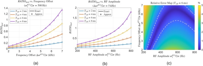
Comparison between the approximated analyticalRATIOdosland its exact numerical solution. (a) The relationship betweenRATIOdoslandΔωd1/2π(2–7kHz) at a fixedω1d1/2πof 500 Hz. For eachT1D(2, 4, 6, and 8 ms), the approximate results (markers) closely match the numerical solution curves (solid lines). (b) The relationship betweenRATIOdoslandω1d1/2π(200–800 Hz) at a fixedΔωd1/2πof 5 kHz. The same agreement between approximate (marker) and exact numerical (solid lines) results is observed. (c) The relative error across theω1d1/2πandΔωd1/2πrange.

Figure4aillustrates the sensitivity of$\textit{RATIO}_{\textit{dosl}}$to$T_{1 D}$. With$\omega_{1}^{d \left(1\right)} / 2 \pi$fixed at 500 Hz and$\Delta \omega^{d \left(1\right)} / 2 \pi$set to 5, 6, and 7 kHz,$\textit{RATIO}_{\textit{dosl}}$increases markedly as$T_{1 D}$rises from 1 to 10 ms, demonstrating high sensitivity. Figure4bdepicts the sensitivity of$\textit{RATIO}_{\textit{dosl}}$to other tissue parameters including$R_{1 a}$,$R_{2 a}$,$R_{1 b}$, MPF,$R$, and$T_{2 b}$.$\textit{RATIO}_{\textit{dosl}}$is essentially independent of$R_{1 a}$,$R_{2 a}$,$R_{1 b}$, and MPF. While it exhibits low sensitivity to the exchange rate$R$and pronounced sensitivity to$T_{2 b}$, these parameters are typically treated as constants in human studies.

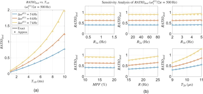
(a) The relationship betweenRATIOdoslandT1Dat fixedω1d1/2π= 500Hz with selectedΔωd1/2π= 5,6, and 7 kHz. Approximate results (markers) closely match numerical solutions (solid lines) overT1D= 1–10 ms. For allΔωd1values,RATIOdoslincreases withT1D, confirming the high sensitivity ofRATIOdosltoT1D. (b) The relationship betweenRATIOdosland other tissue parameters, includingR1a,R2a,R1b, MPF,R, andT2b.

Figure5presents an accuracy analysis of$T_{1 D}$estimation from measured$\textit{RATIO}_{\textit{dosl}}$using analytical estimation method across various spin‐lock parameters ($\Delta \omega^{d \left(1\right)}$,$\omega_{1}^{d \left(1\right)}$, and TSL). Figure5a,dsuggest that$\Delta \omega^{d \left(1\right)} / 2 \pi$values of 3–7 kHz combined with$\omega_{1}^{d \left(1\right)} / 2 \pi$= 500 Hz are optimal, yielding relative errors below 5%. Figure5b,eindicate that$\omega_{1}^{d \left(1\right)} / 2 \pi$values of 500–700 Hz are favorable. The relationship between relative error and TSL varies by$\Delta \omega^{d \left(1\right)}$; notably, at$\Delta \omega^{d \left(1\right)} / 2 \pi$= 5 kHz, the error is nearly independent of TSL. Based on these findings, we selected$\omega_{1}^{d \left(1\right)} / 2 \pi$= 500 Hz,$\Delta \omega^{d \left(1\right)} / 2 \pi$= 5 kHz, and TSL = 80 ms for in vivo experiments. These parameters fall within the scanner's SAR constraints and RF hardware limits.

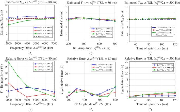
Simulation of the accuracy ofT1Destimation as a function of spin‐lock pulse parameters. (a) EstimatedT1Dversus resonance frequency offset (Δωd1/2π, 2–7 kHz) at fixed TSL = 80 ms and selected spin‐lock field strengthω1d1/2πvalues of 300, 500, and 700 Hz. (b) EstimatedT1Dversus spin‐lock field strength (ω1d1/2π, 200–800 Hz) at fixed TSL = 80 ms and selectedΔωd1/2πvalues of 5, 6, and 7 kHz. (c) EstimatedT1Dversus spin‐lock duration (TSL, 40–120 ms) at fixedω1d1/2π= 500 Hz and selected (Δωd1/2πvalues of 5, 6, and 7 kHz. (d–f) Corresponding relative errors of the estimatedT1Dwith respect to the ground‐truth value. The dashed line in (a–c) indicates the ground‐truthT1D=6.2ms.

Figure6adisplays the dependence of$\textit{RATIO}_{\textit{dosl}}$on$B_{0}$and$B_{1}$inhomogeneity, alongside the relative error compared to the ground truth ($B_{0}$= 0 Hz,$B_{1}$= 1 n.u.). For$B_{0}$between −100 and 100 Hz,$\textit{RATIO}_{\textit{dosl}}$exhibits minimal variation and minor oscillations around the ground truth. However, consistent with theoretical predictions,$\textit{RATIO}_{\textit{dosl}}$is sensitive to$B_{1}$inhomogeneity because the lineshape depends on the actual RF amplitude. Notably, incorporating$B_{1}$maps for retrospective correction of$T_{1 D}$effectively mitigates the impact of this inhomogeneity. As shown in Table1A, the bias in$T_{1 D}$quantification due to field inhomogeneity is significantly reduced following this correction.

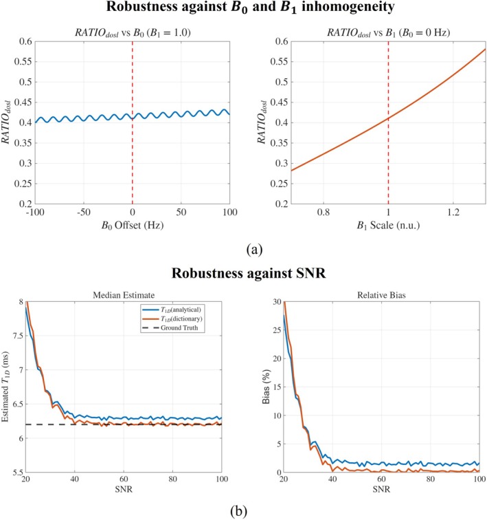
(a) Robustness ofRATIOdosltoB0andB1inhomogeneity, displaying sensitivity toB0offsets (−100 to 100 Hz) andB1scaling factors (0.7 to 1.3 n.u.). (b) Robustness to SNR: a comparison of analytical estimation versus dictionary matching forT1D. The plot shows the median estimate and relative bias compared to the ground‐truthT1D= 6.2ms across an SNR range of 20–100.

Table: Summary of robustness tests forT1Destimation.

Table1Bdetails the results under variations of MT parameters. The mean$\pm$standard deviation of$\textit{RATIO}_{\textit{dosl}}$,$T_{1 D}$(analytical estimation), and$T_{1 D}$(dictionary matching) were$0.41 \pm 0.02$,$6.29 \pm 0.34$, and$6.21 \pm 0.4$ms, respectively. Estimated$T_{1 D}$values show minimal bias (< 0.1 ms) relative to the ground truth (6.2 ms). These findings indicate that, assuming fixed MT parameters (excluding$T_{2 b}$), the estimation of$T_{1 D}$is insensitive to variations in MT parameters.

Figure6bpresents the robustness against SNR. We calculated the median due to the presence of outliers at low SNR and relative bias for the estimated$T_{1 D}$. This analysis confirms that SNR is critical for reliability, indicating that analytical estimation and dictionary matching methods require an SNR of at least ~40 to maintain a relative bias below 3%.

Phantom and In Vivo Studies

Figure7ashows the MPF‐SL acquisitions for the agar and PL161 phantoms. The$R_{\text{mpfsl}}$and the derived MPF are strongly associated with phantom concentration. Figure7bpresents the corresponding$\textit{RATIO}_{\textit{dosl}}$and$T_{1 D}$maps. The$\textit{RATIO}_{\textit{dosl}}$map highlights the contrast of the PL161 phantom, demonstrating its sensitivity to the ihMT effect. In the$T_{1 D}$maps, the long$T_{1 D}$of the PL161 phantom is confirmed by our method, whereas the agar phantom exhibits a notable MPF but negligible$T_{1 D}$, consistent with its lack of dipolar behavior. Figure7c–fshow the relationships of$\textit{RATIO}_{\textit{dosl}}$and$T_{1 D}$with phantom concentration. Both$\textit{RATIO}_{\textit{dosl}}$and$T_{1 D}$show no obvious dependence on PL161 concentration overall.

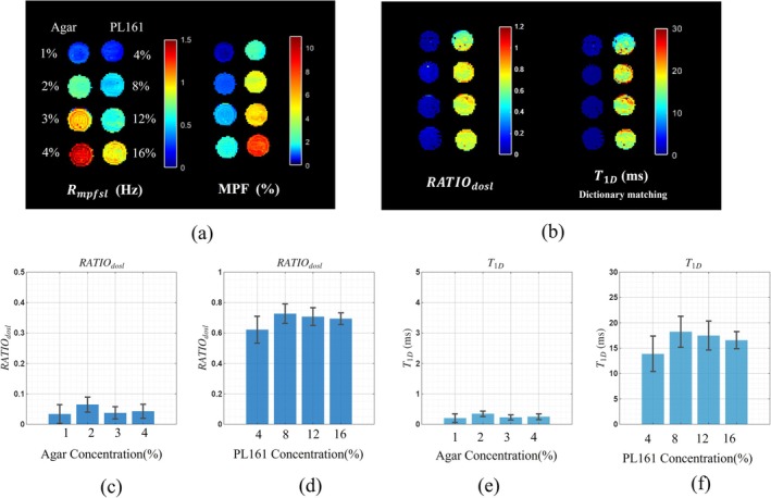
Results of phantom studies. (a)Rmpfsland MPF maps. (b)RATIOdoslandT1Dmap. The first column displays agar phantoms with concentrations of 1%, 2%, 3%, and 4% (from top to bottom); the second column displays PL161 phantoms with concentrations of 4%, 8%, 12%, and 16% (from top to bottom). (c)–(d) Bar plots ofRATIOdoslfor the agar and PL161 phantoms, respectively. Bars represent the mean within each phantom ROI, and error bars represent the standard deviation within ROI. (e)–(f) Corresponding bar plots ofT1D.

Figure8presents in vivo results from one volunteer (V1). The$T_{1}$‐weighted anatomical image for the acquired slices and the 16 major white matter bundles are shown in Figure8a,b. Figure8c,dshow the MPF maps and$\textit{RATIO}_{\textit{dosl}}$maps, which exhibit different contrasts for white matter and indicate that these two parameters may carry different molecular signatures of tissues.$T_{1 D}$maps were derived from the$\textit{RATIO}_{\textit{dosl}}$maps using analytical estimation and dictionary matching, with and without$B_{1}$correction. The resulting$T_{1 D}$maps preserve a contrast similar to that of the$\textit{RATIO}_{\textit{dosl}}$maps (Figure8e–h). Results for the other volunteers are provided inSupporting Information 2. Table2summarizes the mean and standard deviation of MPF,$\textit{RATIO}_{\textit{dosl}}$, and the corresponding$T_{1 D}$across the 16 major white matter fiber bundles in 10 volunteers.

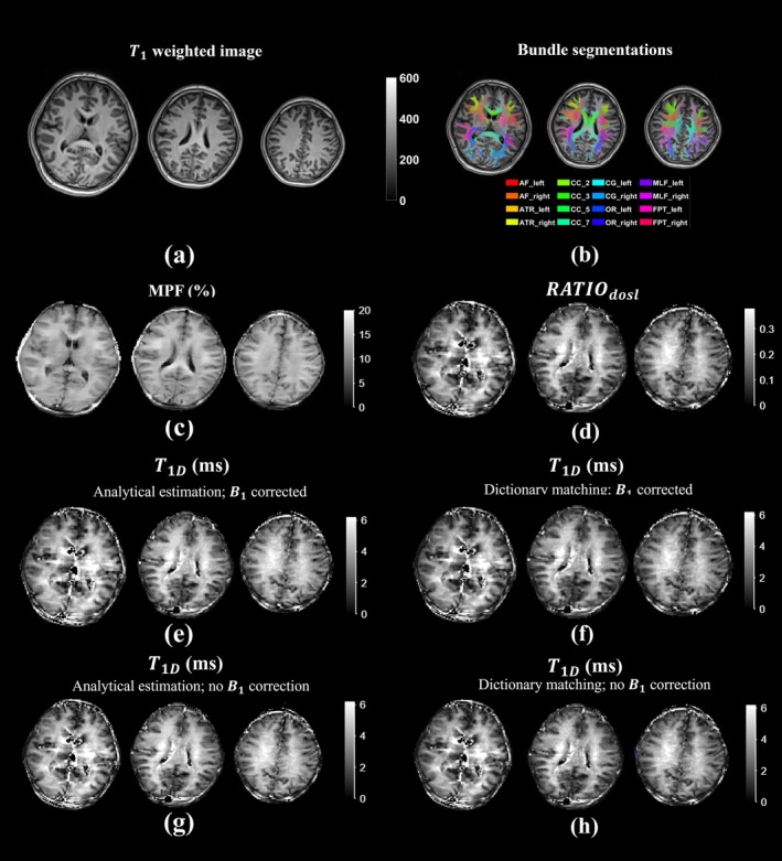
Representative results from one volunteer. (a)T1‐weighted image of the acquired slices. (b) Bundle segmentation showing 16 major white matter fiber bundles. (c) MPF maps derived from MPF‐SL. (d)RATIOdoslmaps. (e)–(f)T1Dmaps obtained via analytical estimation and dictionary matching, respectively, withB1correction. (g)–(h) CorrespondingT1Dmaps obtained via analytical estimation and dictionary matching withoutB1correction.

Table: Mean and standard deviation of MPF,RATIOdosl, andT1Dacross the 16 major white matter fiber bundles.

Discussion

Our proposed framework allows simultaneous quantification of$T_{1 D}$and MPF within a single scan. While MPF primarily reflects macromolecular content,$T_{1 D}$provides complementary sensitivity to microstructural integrity through the ihMT effect. Central to this approach is$\textit{RATI} O_{\textit{dosl}}$, a$T_{1 D}$‐sensitive measure derived from the distinct relaxation rate$R_{\textit{dosl}}$. Estimation of$\textit{RATI} O_{\textit{dosl}}$, and its subsequent conversion to$T_{1 D}$with$B_{1}$correction, can be achieved using only three spin‐lock‐prepared images. Notably, two of these images can also be used for MPF quantification. Consequently, this simultaneous mapping strategy enables characterization of both tissue microstructure and macromolecular content within a single rapid scan. Recently, Hertanu et al. compared ihMTR and MPF with diffusion‐based modeling to investigate the microstructural correlates of white and gray matter [39]. Their findings highlight the potential of these parameters to disentangle distinct tissue mechanisms, supporting the premise that combined assessment of MPF and$T_{1 D}$may enhance tissue characterization. Accordingly, the proposed method may facilitate further clinical investigation of these parameters across a range of pathologies, both in the brain and in other organ systems.

In previous studies, Varma et al. reported an in vivo white matter$T_{1 D}$value of approximately 6.2 ms using a multi‐ihMTR approach [6] and approximately 3 ms under the assumption of a single MT compartment with a single$T_{1 D}$[11], whereas West et al. reported white matter$T_{1 D}$values of approximately 3.5–5.5 ms using an MRF‐based technique [20]. In the present study, we obtained white matter$T_{1 D}$values in the range of approximately 3.70–4.80 ms. Although these values are broadly consistent with prior reports, precise validation of the true$T_{1 D}$remains challenging. Moreover, the sensitivity of our method to$T_{2 b}$may introduce potential bias in the estimated$T_{1 D}$, which could also contribute to differences relative to prior reports. To provide indirect support for our$T_{1 D}$estimates, we performed in vivo experiments in which the$T_{s}$of the dual frequency spin‐lock preparation was varied from 0.5 to 20 ms. The results showed that white matter was strongly highlighted when the dual‐frequency spin‐lock$T_{s}$was ≤ 4 ms (FigureS1.2inSupporting Information 1), which provides indirect support for the obtained$T_{1 D}$values based on the expected$T_{1 D}$‐filtering effect.

For the proposed method, because$\textit{RATIO}_{\textit{dosl}}$is derived from different$R_{1 \rho}$measurements under a constant spin‐lock field direction, contributions from the water pool are effectively cancelled. Simulation studies further indicate that$\textit{RATIO}_{\textit{dosl}}$exhibits only weak dependence on other MT parameters (e.g., MPF, R, and R1b).

Prolonged scan times often limit the clinical utility of$T_{1 D}$assessment [6,20]. Our approach addresses this by requiring only three spin‐lock prepared images for joint$T_{1 D}$and MPF quantification. Although this study demonstrated the technique in 2D slices, extending the method to whole‐brain coverage is feasible using fast 3D MRI acquisition strategies [40,41,42]. In previous work [42], using four spin‐lock prepared images combined with 3D FSE/TSE acquisition, whole‐brain coverage of$T_{1 \rho}$quantification could be achieved within 5 min. Consequently, by leveraging strategies that rely solely on three spin‐lock prepared images, we estimate the proposed method can achieve whole‐brain coverage in 5 min.

Our method employs the least negative eigenvalue to model signal evolution, an approach traditionally assumed to necessitate long saturation times [29]. However, our analysis indicates that this approximation remains robust at short spin‐lock durations (e.g., 80 ms) under specific experimental conditions. By utilizing large frequency offsets relative to the spin‐lock amplitude$\left(\Delta \omega \gg \omega_{1}\right)$, the system enters a regime where magnetization decay is dominated by a single component. In this context, contributions from faster‐decaying modes are negligible, allowing the least negative eigenvalue to characterize signal evolution as a mono‐exponential process. Moreover, at the large frequency offset used in this study ($\Delta \omega^{d \left(1\right)} / 2 \pi$=5kHz), CEST and NOE contributions are expected to be negligible [23]. In addition, three‐pool simulations that explicitly incorporated a CEST pool showed negligible effects on$\textit{RATIO}_{\textit{dosl}}$across broad CEST parameter ranges (FigureS1.3inSupporting Information 1).

In MT imaging, saturation efficiency is strongly influenced by the time‐averaged RF power, which is proportional to the time‐averaged$B_{1}^{2}$. Under the same peak‐power and SAR constraints, a piecewise‐constant RF waveform may provide higher effective average saturation than a conventional Gaussian RF pulse. Moreover, piecewise‐constant RF irradiation is more readily incorporated into the Provotorov formalism. In conventional saturation‐based methods, however, the use of square‐wave RF irradiation is associated with a trade‐off involving direct water saturation, partly because of its broader spectral characteristics. By contrast, in the proposed spin‐lock‐based framework, square‐wave RF pulses can be incorporated into the preparation process in a manner that is less constrained by this trade‐off.

In this study, we compared analytical estimation and dictionary matching for$T_{1 D}$quantification. At SNR$\geq 40$, both approaches yielded low error; analytical estimation showed a small residual bias due to model approximations, whereas dictionary matching achieved slightly higher accuracy. Analytical estimation offers fast computation without the memory and runtime overhead associated with large dictionaries; however, its accuracy can depend on careful optimization of acquisition parameters to control bias across tissue types. Dictionary matching is, in principle, applicable to arbitrary acquisition settings. Overall, the choice of$T_{1 D}$estimation approach should be guided by the study's SNR conditions and acquisition design.

Beyond quantitative$T_{1 D}$mapping, the proposed framework may also be adapted for$T_{1 D}$‐weighted contrast generation. Because the contrast mechanism depends on the relationship between the switching time$T_{s}$and the underlying$T_{1 D}$, adjustment of$T_{s}$may enable preferential sensitivity to components with short, intermediate, or long$T_{1 D}$values. In such cases, simple approximate metrics derived from a limited number of images, for example$\left(M_{s}^{\left(1\right)} - M_{d}^{\left(1\right)}\right) / M_{d}^{\left(1\right)}$, may offer a practical alternative to explicit$T_{1 D}$quantification. This strategy may be useful in applications where the primary goal is to enhance$T_{1 D}$‐dependent contrast rather than to obtain absolute parametric estimates. Further work is needed to optimize and validate such acquisition schemes for selective component weighting.

Looking ahead, other spin‐lock‐based quantitative MT techniques, such as pulsed spin‐lock approaches [25], may also be leveraged for dipolar‐order quantification. Pulsed spin‐lock methods can mitigate RF hardware limitations, offering particular benefits for body imaging and low‐field applications where power constraints are pronounced.

Although our theoretical analysis and experimental results support the reliability and clinical feasibility of spin‐lock–based$T_{1 D}$quantification, several areas warrant further investigation to refine the technique:

Conclusions

We demonstrated a novel and rapid off‐resonance spin‐lock technique for quantifying the dipolar relaxation time$T_{1 D}$. The ability to measure both MPF and$T_{1 D}$within a single scan highlights the potential clinical utility of this approach and provides a promising pathway toward integrating molecular microstructural imaging into clinical practice.

Author Contributions

Zijian Gao:conceptualization, data curation, software, investigation, methodology, project administration, writing – original draft, visualization.Qianxue Shan:investigation, methodology, formal analysis, validation.Ziqin Zhou:data curation, resources, software.Ziqiang Yu:data curation, software, methodology.Weitian Chen:conceptualization, investigation, project administration, supervision, methodology, funding acquisition, writing – review and editing.

Conflicts of Interest

Weitian Chen is a shareholder of Illuminatio Medical Technology Limited.

Acknowledgments

This study was supported by a grant from the Research Grants Council of the Hong Kong SAR (Project GRF 14213322).

Data Availability Statement

The data that support the findings of this study are available on request from the corresponding author. The data are not publicly available due to privacy or ethical restrictions.

Associated Data

Data Availability Statement

The data that support the findings of this study are available on request from the corresponding author. The data are not publicly available due to privacy or ethical restrictions.

References

1. Goldman M., Spin Temperature and Nuclear Magnetic Resonance in Solids (Clarendon Press, 1970).
2. Yeung H. N., Adler R. S., and Swanson S. D., “Transient Decay of Longitudinal Magnetization in Heterogeneous Spin Systems Under Selective Saturation. IV. Reformulation of the Spin‐Bath‐Model Equations by the Redfield‐Provotorov Theory,” Journal of Magnetic Resonance. Series A 106, no. 1 (1994): 37–45, 10.1006/jmra.1994.1004. doi.org/10.1006/jmra.1994.1004
3. Morrison C., Stanisz G., and Henkelman R. M., “Modeling Magnetization Transfer for Biological‐Like Systems Using a Semi‐Solid Pool With a Super‐Lorentzian Lineshape and Dipolar Reservoir,” Journal of Magnetic Resonance. Series B 108, no. 2 (1995): 103–113, 10.1006/jmrb.1995.1111. doi.org/10.1006/jmrb.1995.1111
4. Varma G., Duhamel G., de Bazelaire C., and Alsop D. C., “Magnetization Transfer From Inhomogeneously Broadened Lines: A Potential Marker for Myelin,” Magnetic Resonance in Medicine 73, no. 2 (2015): 614–622, 10.1002/mrm.25174. doi.org/10.1002/mrm.25174
5. Manning A. P., Chang K. L., MacKay A. L., and Michal C. A., “The Physical Mechanism of “Inhomogeneous” Magnetization Transfer MRI,” Journal of Magnetic Resonance 274 (2017): 125–136, 10.1016/j.jmr.2016.11.013. doi.org/10.1016/j.jmr.2016.11.013
6. Varma G., Girard O. M., Prevost V. H., Grant A. K., Duhamel G., and Alsop D. C., “In Vivo Measurement of a New Source of Contrast, the Dipolar Relaxation Time, T1D, Using a Modified Inhomogeneous Magnetization Transfer (ihMT) Sequence,” Magnetic Resonance in Medicine 78, no. 4 (2017): 1362–1372, 10.1002/mrm.26523. doi.org/10.1002/mrm.26523
7. Alsop D. C., Ercan E., Girard O. M., et al., “Inhomogeneous Magnetization Transfer Imaging: Concepts and Directions for Further Development,” NMR in Biomedicine 36, no. 6 (2023): e4808, 10.1002/nbm.4808. doi.org/10.1002/nbm.4808
8. Van Obberghen E., Mchinda S., le Troter A., et al., “Evaluation of the Sensitivity of Inhomogeneous Magnetization Transfer (ihMT) MRI for Multiple Sclerosis,” AJNR. American Journal of Neuroradiology 39, no. 4 (2018): 634–641, 10.3174/ajnr.A5563. doi.org/10.3174/ajnr.A5563
9. Geeraert B. L., Lebel R. M., Mah A. C., et al., “A Comparison of Inhomogeneous Magnetization Transfer, Myelin Volume Fraction, and Diffusion Tensor Imaging Measures in Healthy Children,” NeuroImage 182 (2018): 343–350, 10.1016/j.neuroimage.2017.09.019. doi.org/10.1016/j.neuroimage.2017.09.019
10. van der Weijden C. W. J., Biondetti E., Gutmann I. W., et al., “Quantitative Myelin Imaging With MRI and PET: An Overview of Techniques and Their Validation Status,” Brain: A Journal of Neurology 146, no. 4 (2023): 1243–1266, 10.1093/brain/awac436. doi.org/10.1093/brain/awac436
11. Varma G., Girard O. M., Prevost V. H., Grant A. K., Duhamel G., and Alsop D. C., “Interpretation of Magnetization Transfer From Inhomogeneously Broadened Lines (ihMT) in Tissues as a Dipolar Order Effect Within Motion Restricted Molecules,” Journal of Magnetic Resonance 260 (2015): 67–76, 10.1016/j.jmr.2015.08.024. doi.org/10.1016/j.jmr.2015.08.024
12. Prevost V. h., Girard O. m., Mchinda S., Varma G., Alsop D. c., and Duhamel G., “Optimization of Inhomogeneous Magnetization Transfer (ihMT) MRI Contrast for Preclinical Studies Using Dipolar Relaxation Time (T1D) Filtering,” NMR in Biomedicine 30, no. 6 (2017): e3706, 10.1002/nbm.3706. doi.org/10.1002/nbm.3706
13. Hertanu A., Soustelle L., Le Troter A., et al., “T1D‐Weighted ihMT Imaging – Part I. Isolation of Long‐ and Short‐T1D Components by T1D‐Filtering,” Magnetic Resonance in Medicine 87, no. 5 (2022): 2313–2328, 10.1002/mrm.29139. doi.org/10.1002/mrm.29139
14. Hertanu A., Soustelle L., Buron J., et al., “T1D‐Weighted ihMT Imaging – Part II. Investigating the Long‐ and Short‐T1D Components Correlation With Myelin Content. Comparison With R1 and the Macromolecular Proton Fraction,” Magnetic Resonance in Medicine 87, no. 5 (2022): 2329–2346, 10.1002/mrm.29140. doi.org/10.1002/mrm.29140
15. Varma G., Fanny M., Girard O., Duhamel G., and Alsop D., “An Inhomogeneous Magnetization Transfer (ihMT) Quantification Method Robust to B1 and T1 Variations in Magnetization Prepared Acquisitions,” ISMRM 27th Annual Meeting, Montreal, 2019, p4911.
16. Zhang L., Chen T., Tian H., et al., “Reproducibility of Inhomogeneous Magnetization Transfer (ihMT): A Test‐Retest, Multi‐Site Study,” Magnetic Resonance Imaging 57 (2019): 243–249, 10.1016/j.mri.2018.11.010. doi.org/10.1016/j.mri.2018.11.010
17. Hou G., Lai W., Jiang W., et al., “Myelin Deficits in Patients With Recurrent Major Depressive Disorder: An Inhomogeneous Magnetization Transfer Study,” Neuroscience Letters 750 (2021): 135768, 10.1016/j.neulet.2021.135768. doi.org/10.1016/j.neulet.2021.135768
18. Chen G., Fu S., Chen P., et al., “Reduced Myelin Density in Unmedicated Major Depressive Disorder: An Inhomogeneous Magnetization Transfer MRI Study,” Journal of Affective Disorders 300 (2022): 114–120, 10.1016/j.jad.2021.12.111. doi.org/10.1016/j.jad.2021.12.111
19. Malik S. J., Teixeira R. P. A. G., West D. J., Wood T. C., and Hajnal J. V., “Steady‐State Imaging With Inhomogeneous Magnetization Transfer Contrast Using Multiband Radiofrequency Pulses,” Magnetic Resonance in Medicine 83, no. 3 (2020): 935–949, 10.1002/mrm.27984. doi.org/10.1002/mrm.27984
20. West D. J., Cruz G., Teixeira R. P. A. G., et al., “An MR Fingerprinting Approach for Quantitative Inhomogeneous Magnetization Transfer Imaging,” Magnetic Resonance in Medicine 87, no. 1 (2022): 220–235, 10.1002/mrm.28984. doi.org/10.1002/mrm.28984
21. Soustelle L., Mchinda S., Hertanu A., et al., “Inhomogeneous Magnetization Transfer (ihMT) Imaging Reveals Variable Recovery Profiles of Active MS Lesions According to Size and Localization,” Imaging Neuroscience 2 (2024): imag‐2‐00235, 10.1162/imag_a_00235. doi.org/10.1162/imag_a_00235
22. Lebel C. and Deoni S., “The Development of Brain White Matter Microstructure,” NeuroImage 182 (2018): 207–218, 10.1016/j.neuroimage.2017.12.097. doi.org/10.1016/j.neuroimage.2017.12.097
23. Hou J., Wong V. W., Jiang B., et al., “Macromolecular Proton Fraction Mapping Based on Spin‐Lock Magnetic Resonance Imaging,” Magnetic Resonance in Medicine 84, no. 6 (2020): 3157–3171, 10.1002/mrm.28362. doi.org/10.1002/mrm.28362
24. Hou J., Wong V. W. S., Qian Y., et al., “Detecting Early‐Stage Liver Fibrosis Using Macromolecular Proton Fraction Mapping Based on Spin‐Lock MRI: Preliminary Observations,” Journal of Magnetic Resonance Imaging 57, no. 2 (2023): 485–492, 10.1002/jmri.28308. doi.org/10.1002/jmri.28308
25. Shan Q., Yu Z., Jiang B., et al., “Quantitative Macromolecular Proton Fraction Imaging Using Pulsed Spin‐Lock,” Magnetic Resonance in Medicine 94 (2025): 2492–2507, 10.1002/mrm.70021. doi.org/10.1002/mrm.70021
26. Gao Z., Yu Z., Zhou Z., et al., “Orientation‐Independent Quantification of Macromolecular Proton Fraction in Tissues With Suppression of Residual Dipolar Coupling,” NMR in Biomedicine 38, no. 1 (2025): e5293, 10.1002/nbm.5293. doi.org/10.1002/nbm.5293
27. Gao Z., Zhou Z., Yu Z., et al., “Orientation‐Independent Magnetization Transfer Imaging of Brain White Matter,” NeuroImage 320 (2025): 121456, 10.1016/j.neuroimage.2025.121456. doi.org/10.1016/j.neuroimage.2025.121456
28. Morrison C. and Henkelman M. R., “A Model for Magnetization Transfer in Tissues,” Magnetic Resonance in Medicine 33, no. 4 (1995): 475–482, 10.1002/mrm.1910330404. doi.org/10.1002/mrm.1910330404
29. Zaiss M., Zu Z., Xu J., et al., “A Combined Analytical Solution for Chemical Exchange Saturation Transfer and Semi‐Solid Magnetization Transfer: An Analytical Solution for CEST and MT,” NMR in Biomedicine 28, no. 2 (2015): 217–230, 10.1002/nbm.3237. doi.org/10.1002/nbm.3237
30. Trott O. and Palmer A. G., “R1ρ Relaxation Outside of the Fast‐Exchange Limit,” Journal of Magnetic Resonance 154, no. 1 (2002): 157–160, 10.1006/jmre.2001.2466. doi.org/10.1006/jmre.2001.2466
31. Yarnykh V. L., “Pulsed Z‐Spectroscopic Imaging of Cross‐Relaxation Parameters in Tissues for Human MRI: Theory and Clinical Applications,” Magnetic Resonance in Medicine 47, no. 5 (2002): 929–939, 10.1002/mrm.10120. doi.org/10.1002/mrm.10120
32. Yarnykh V. L., “Fast Macromolecular Proton Fraction Mapping From a Single Off‐Resonance Magnetization Transfer Measurement,” Magnetic Resonance in Medicine 68, no. 1 (2012): 166–178, 10.1002/mrm.23224. doi.org/10.1002/mrm.23224
33. Hou J., Cai Z., Chen W., and So T. Y., “Spin‐Lock Based Fast Whole‐Brain 3D Macromolecular Proton Fraction Mapping of Relapsing–Remitting Multiple Sclerosis,” Scientific Reports 14, no. 1 (2024): 17943, 10.1038/s41598-024-67445-4. doi.org/10.1038/s41598-024-67445-4
34. Stanisz G. J., Odrobina E. E., Pun J., et al., “T1, T2 Relaxation and Magnetization Transfer in Tissue at 3T,” Magnetic Resonance in Medicine 54, no. 3 (2005): 507–512, 10.1002/mrm.20605. doi.org/10.1002/mrm.20605
35. Assländer J., Mao A., Marchetto E., et al., “Unconstrained Quantitative Magnetization Transfer Imaging: Disentangling T1 of the Free and Semi‐Solid Spin Pools,” Imaging Neuroscience 2 (2024): 1–16, 10.1162/imag_a_00177. doi.org/10.1162/imag_a_00177
36. Sled J. G. and Pike G. B., “Quantitative Interpretation of Magnetization Transfer in Spoiled Gradient Echo MRI Sequences,” Journal of Magnetic Resonance 145, no. 1 (2000): 24–36, 10.1006/jmre.2000.2059. doi.org/10.1006/jmre.2000.2059
37. Swanson S. D., Malyarenko D. I., Fabiilli M. L., Welsh R. C., Nielsen J. F., and Srinivasan A., “Molecular, Dynamic, and Structural Origin of Inhomogeneous Magnetization Transfer in Lipid Membranes,” Magnetic Resonance in Medicine 77, no. 3 (2017): 1318–1328, 10.1002/mrm.26210. doi.org/10.1002/mrm.26210
38. Wasserthal J., Neher P., and Maier‐Hein K. H., “TractSeg ‐ Fast and Accurate White Matter Tract Segmentation,” NeuroImage 183 (2018): 239–253, 10.1016/j.neuroimage.2018.07.070. doi.org/10.1016/j.neuroimage.2018.07.070
39. Hertanu A., Pavan T., Uhl Q., Mezzano S., Feiweier T., and Jelescu I. O., “Microstructural Correlates of White and Gray Matter in the Healthy Human Brain: Comparative Analysis of Diffusion Biophysical Models, Inhomogeneous Magnetization Transfer, and Macromolecular Proton Fraction,” December 2025, 2025.12.06.692761, 10.64898/2025.12.06.692761. doi.org/10.64898/2025.12.06.692761
40. Chen W., Takahashi A., and Han E.. “3D Quantitative Imaging of T1rho and T2,” ISMRM 19th Annu Meet Montr. 2011. P231.
41. Jordan C. D., McWalter E. J., Monu U. D., et al., “Variability of CubeQuant T1ρ, Quantitative DESS T2, and Cones Sodium MRI in Knee Cartilage,” Osteoarthritis and Cartilage 22, no. 10 (2014): 1559–1567, 10.1016/j.joca.2014.06.001. doi.org/10.1016/j.joca.2014.06.001
42. Villanueva‐Meyer J. E., Barajas R. F., Mabray M. C., et al., “Differentiation of Brain Tumor‐Related Edema Based on 3D T1rho Imaging,” European Journal of Radiology 91 (2017): 88–92, 10.1016/j.ejrad.2017.03.022. doi.org/10.1016/j.ejrad.2017.03.022
43. Sled J. G. and Pike G. B., “Quantitative Imaging of Magnetization Transfer Exchange and Relaxation Properties In Vivo Using MRI,” Magnetic Resonance in Medicine 46, no. 5 (2001): 923–931, 10.1002/mrm.1278. doi.org/10.1002/mrm.1278
44. Yarnykh V. L. and Yuan C., “Cross‐Relaxation Imaging Reveals Detailed Anatomy of White Matter Fiber Tracts in the Human Brain,” NeuroImage 23, no. 1 (2004): 409–424, 10.1016/j.neuroimage.2004.04.029. doi.org/10.1016/j.neuroimage.2004.04.029
45. Davies G. R., Tozer D. J., Cercignani M., et al., “Estimation of the Macromolecular Proton Fraction and Bound Pool T2 in Multiple Sclerosis,” Multiple Sclerosis Journal 10, no. 6 (2004): 607–613, 10.1191/1352458504ms1105oa. doi.org/10.1191/1352458504ms1105oa
46. Carvalho V. N. D., Hertanu A., Grélard A., et al., “MRI Assessment of Multiple Dipolar Relaxation Time (T1D) Components in Biological Tissues Interpreted With a Generalized Inhomogeneous Magnetization Transfer (ihMT) Model,” Journal of Magnetic Resonance 311 (2020): 106668, 10.1016/j.jmr.2019.106668. doi.org/10.1016/j.jmr.2019.106668
47. Lam M. H., Novoselova M., Yung A., et al., “Interpretation of Inhomogeneous Magnetization Transfer in Myelin Water Using a Four‐Pool Model With Dipolar Reservoirs,” Magnetic Resonance in Medicine 94, no. 1 (2025): 278–292, 10.1002/mrm.30465. doi.org/10.1002/mrm.30465
48. Morris S. R., Frederick R., MacKay A. L., Laule C., and Michal C. A., “Orientation Dependence of Inhomogeneous Magnetization Transfer and Dipolar Order Relaxation Rate in Phospholipid Bilayers,” Journal of Magnetic Resonance 338 (2022): 107205, 10.1016/j.jmr.2022.107205. doi.org/10.1016/j.jmr.2022.107205

---

Republished from the open web under CC-BY. Authors: Gao Z, Shan Q, Zhou Z, Yu Z, Chen W. Read the original.