Simultaneous learning of static and dynamic charges.

Introduction

Electric fields influence the structure, dynamics, and reactivity of molecular and condensed-phase systems. Processes such as catalysis, charge transport, or characterization techniques like infrared (IR) spectroscopy depend sensitively on how atoms respond to internal and external electric fields.1–3First-principles electronic-structure methods capture these responses with high accuracy, but their computational cost limits their use for large, heterogeneous systems or long simulation times. Machine-learned interatomic potentials (MLIPs) have begun to address this challenge by providing near-quantum-chemical accuracy for the structure and dynamics of molecules and condensed phases at drastically reduced cost.4Modern architectures—often graph neural networks with equivariant message-passing—effectively model complex many-atom correlations, albeit within a finite interaction range and model capacity.5–8However, most MLIPs remain restricted to field-free simulations: they do not natively incorporate the effects of external fields or predict electrical response properties, limiting their applicability in technologically relevant scenarios.

Several strategies have been developed to endow MLIPs with electric-field awareness. One class of methods learns dipoles or local dipole contributions,9–14but these approaches face fundamental challenges: for periodic systems, dipoles are defined onlymoduloa polarization quantum,12,15,16which requires care during training, as the loss function must account for this multi-valuedness. Other approaches bypass these issues by learning scalar effective charges17,18or tensorial quantities such as Born effective charges (BECs), also called atomic polar tensors (APTs).19–21These models couple external fields to learned charges, generating auxiliary field-dependent forces and thus avoid the conceptual ambiguities of polarization-based methods. BEC-based models perform well in capturing the linear electric response. However, these models typically neglect an important physical ingredient: the external electric-field response of atoms is intimately linked to the electrostatic interaction between atoms. Effective charges used to model long-range Coulomb forces reflect internally screened interactions, whereas BECs describe the unscreened response of the electron density to an external field. Crucially, the distinction between internal (screened) and external (unscreened) responses becomes pronounced in heterogeneous systems such as clusters, interfaces, or molecular mixtures, where assuming a single homogeneous screening value may not be sufficient.

Besides electric-field response, long-range electrostatics have already been incorporated in MLIPs using fixed charges,22,23ML-fitted surrogate charges such as Hirshfeld charges,24,25dipole-matching schemes,26or global charge-equilibration networks.17,18,27,28Recently, differentiable Ewald summation frameworks29,30have enabled end-to-end charge learning, removing ambiguities in charge assignment.31–33A few recent studies attempt to combine long-range electrostatics with electric-field response, for example by deriving BECs from end-to-end learned internal charges.34,35These approaches generally assume homogeneous isotropic screening, which can provide decent qualitative behaviour in bulk systems but may fail in heterogeneous environments, limiting their applicability for general-purpose ML potentials.

This breakdown raises a central open question: should static (effective) and dynamic (BEC) charges be learned together, constrained by their physical relationship, or treated as independent quantities? Here, we address this question by systematically evaluating both coupled and uncoupled strategies in long-range ML architectures, including cases with environment-dependent screening, to clarify where and why homogeneous screening assumptions break down and how accuracy can be restored. We critically compare different models in terms of accuracy, interpretability, and computational cost, using high-quality finite-field reference data for bulk water as a prototypical polar liquid with well-characterized experimental reference data including IR spectra36and water clusters. Water clusters are of direct scientific relevance as precursors of atmospheric ice-nucleating particles37and as models for aerosol droplets in the context of airborne pathogen transmission.38

Theory and models

Static and dynamic charges

A key concept for describing the response of atomistic systems to externally applied fields is the BEC (or APT) of an atom, which is definedvia19,20

where Created by potrace 1.16, written by Peter Selinger 2001-2019 αis theα-component of the system polarization density,rβitheβ-component of the position of atomi,Vis the system volume,Fβithe force on atomiandEαan externally applied field. The symbolsα,β∈ {x,y,z} specify Cartesian components of the tensors. The right-hand side ofeqn (1)motivates the use of these charges for describing electrostatic interactions with external fields, as it represents the corresponding linear-response coefficient—the change in force induced by an applied external field.

We consider for the moment non-periodic systems, where we define partial chargesqIRithat reproduce the polarizationP= Created by potrace 1.16, written by Peter Selinger 2001-2019 V,

This allows us to relate BECsZito static chargesqIRithrough39

where the first term mimics the “static charges”qIRi, which are sometimes also referred to as the “IR charge” (as it reproduces the system's dipole and thus yields the infrared spectrum, as we will discuss below). The second term ineqn (3)describes the charge flux: the change in the dipole moment due to a collective alteration of the charge distribution as thei-th atom is displaced by an infinitesimal amount. BecauseZiencodes these charge redistribution effects, BECs are also called “dynamic charges”.

Long-ranged machine learned potentialsvialearned static charges

As briefly explained in the introduction, a wide range of methods have been proposed for assigning partial “static” charges to nuclei from the continuous electron density. Popular schemes include Mulliken charges,40Hirshfeld charges33and the aforementioned IR charges.39Each of these methods corresponds to a different definition of the partial charges, and there is no unequivocally “best” choice. Given this ambiguity, it is perhaps not too surprising that many different schemes have been used with similar success to capture long-ranged electrostatic interactions in machine-learned interatomic potentials, including the explicit learning of atomic partial charges,24,25the learning of the position of Wannier centers41and charge equilibration schemes that allow for self-consistent redistribution of atomic charges.27Atomic charges can also be treated simply as fitting parameters to reproduce quantum mechanical energies and forces. This approach is common in classical forcefields.42It is also used implicitly by schemes such as LODE, where long-range descriptors have fitting coefficients that correspond to charge multipoles.43Recently, the latent Ewald summation framework has popularized this strategy for end-to-end charge learning.29Instead of targeting a specific charge partitioning scheme, we focus here on the concept of learned pseudo chargesqi. These are not fitted to any particular definition of atomic charges. Learning static charges indirectly avoids the need to choose an arbitrary partitioning scheme. The model is thus free to infer per-atom quantitiesqi(ξi) that minimize errors in predicted energies, forces, and, where applicable, Born effective charges (BECs). The model uses descriptorsξiof the local environment of each atomiwithin a finite cutoff [seeFig. 1(A) and (B)]. These descriptors are used to predict both the short-range part of the potentialUsriand the atomic pseudo-chargesqi. The pseudo-charges are then used to compute the electrostatic potential and thus ultimately the long-range part of the MLIP. One can go even further and use more general functional forms that do not allow for a transparent interpretation ofqias atomic static charges. This approach, briefly introduced in the following section, has been shown to further improve the accuracy of energies and forces.44

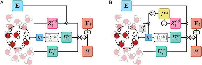
Schematic illustration of the two different model architectures. (A) Shows the architecture of an “uncoupled model”, where BECsZand static chargesqare treated independent of one another. (B) Shows a coupled architecture where the learned pseudo chargesqiare related to the BECs through the polarizationP, with either a globalγθi= const. or local screening parametersγθi. The final output of each model is the total force per atomFiand the electrostatic enthalpyH(seeeqn (11)), which reduces to the internal energyH=Uin the case of no external fields,E= 0.

Uncoupled static/dynamic charge prediction

In the present work, the long-ranged contribution to the potential is constructed using learned pseudo-chargesqiintroduced above. Without PBC, the electrostatic potential

is computed through an automatically differentiable (AD) Coulomb solver. Periodic image contributions are handledviaan AD implementation of the Ewald summation.30To integrate the interactions associated with the Coulomb potential into an energy-decomposable MLIP, we express the long-range energy as

Beyond this physical definition ofUlr, we also consider a more flexible long-range formulation introduced by us in ref.44. Here, the electrostatic potential is processed by a learnable functionfθ, yielding

This modification, referred to as “long-range representations with equivariant messages” (LOREM) has been shown to significantly reduce errors across multiple prediction tasks.44We note that in this work we restrict the architectures to learned scalar pseudo charges only, as opposed to the more general equivariant tensorial pseudo charges proposed in ref.44. When the learnable function is set to beV({qj,rj}j)qi, the model reduces toeqn (5)and retains interpretability of the pseudo charges. We refer to this latter version as the physical long-range architecture.

The simplest extension of long-ranged MLIPs to also predict BECs is to treat them as independent outputs without connection to the static pseudo charges. An architecture capable of this is shown inFig. 1A. Here, the pseudo chargesqi(ξi) are predicted solely for computingUlr, while the BECs constitute a second, independent prediction target derived from the same local environment representationξi. This design allows the model to learn static and dynamic charge responses separately, without enforcing any explicit relation between them.

Because we employ an equivariant descriptorξi, predictingZibecomes straightforward. To obtain the Born effective charge tensorZαβifrom the local atomic environment, we map the equivariant spherical-harmonic features of each atom through a small neural module. The descriptor (restricted to features up to two angular channels) is first processed by several dense layers applied to the spherical channels. An equivariant tensor-coupling step based on Clebsch–Gordan coefficients mixes the angular components to form all symmetry-allowed rank-2 contributions, which are subsequently linearly recombined into a 3 × 3 matrix, which is fitted to BEC labels derived from DFT (see Methods Section 5.1).45This construction ensures that the predicted tensors transform correctly under rotations. Such an approach is essentially the extension of previous works19,46to long-ranged architectures.

Coupled static/dynamic charge prediction

A second possible strategy is to attempt to approximate the infrared chargesqIRiviathe learned pseudo chargesqi(ξi) to constructZiviaeqn (1) and (3), as has been proposed in recent works.34,35,47However, whenqi(ξi) are learned through minimization of energy and force errors usingeqn (4) and (5), these quantities already include screening effects from the instantaneously responding electronic background. For homogeneous bulk systems34or isolated molecules in vacuum,35the screening can be approximated as homogeneous and isotropic. This leads to a simple proportionality between learned and infrared charges

Here, the coupling parameterγcan be interpreted in terms of the high-frequency dielectric permittivity,.34,48,49The underlying assumption of the latter relation is that learned pseudo charges correspond to physically interpretable partial charges and has been shown to allow fora posterioriprediction ofZiin a large variety of systems, if one assumesε∞between 1 (isolated molecules) and 1.83 (bulk water).34,35Here, we will refrain from interpreting the screening parameter as directly related toε∞. Instead, we simply treatγas a learnable parameter that scales the learned pseudo charges to infrared charges. This scaling is determined by requiring that the resulting charges reproduce BEC targets obtained from DFT calculations. However, as we will show below, the assumptions of homogeneous and isotropic screening break down in inhomogeneous environments such as interfaces, where the dielectric response is well known to become both anisotropic and spatially varying.50–53A simple way to resolve the homogeneity assumption is to introduce a local screening factor,

where the scalar coefficientγiis predicted from the local environmentξi, which follows smoothly fromeqn (7). This local formulation captures spatial inhomogeneities, but it still enforces isotropic screening. Promotingγito a tensorial, environment-dependent quantity would be equivalent to directly predicting the full dynamic chargeZi. Consequently, uncoupled learning ofZicaptures both anisotropy and inhomogeneity, whereas scalar local screening only accounts for the latter.

Using the proposed coupling relationseqn (7) and (8)to predictZiviaeqn (3)is the basis for the second family of MLIPs that we study, the coupled models. These models, shown inFig. 1B, use the predictedqi(ξi) to construct the BECs. We explore two variants of these coupled models. (i) In the coupled, global approach, the MLIP is first trained only on energies and forces. Afterwards, a single global screening parameterγ(seeeqn (7)) is fitteda posteriorito minimize the BEC error on the validation set. We intend this strategy to closely follow the strategy of ref.34and35. (ii) In the coupled, local approach, we drop the assumption of a uniform screening factor. Instead, the model predicts a local, environment-dependentγi(seeeqn (8)), learned jointly with energies, forces, and BEC labels. This allows us to test whether relaxing the homogeneity assumption improves BEC prediction accuracy, especially in inhomogeneous systems.

For all coupled architectures an issue arises when incorporating periodic boundary conditions. A naive definition of the polarization densityviaeqn (2) and (7)can result in ill-defined values, due to the periodic boundaries. This problem can be mitigated in molecular systems by learning molecular dipole contributions,54but this approach is incompatible with the atom-centered, point-charge picture adopted by the models we consider in the present work. Zhonget al.34solved this by utilizing an artificial complex phase. We instead calculateZifrom the learned pseudo chargesviatheir positions by

where the index PBC accounts for periodic boundary conditions when computing the distances. We explain the motivation behindeqn (9)in detail in Section SI of the SI.Eqn (9)directly follows from recognizing that for neutral systemsPis translationally invariant and can thus always be formulated with respect to particle distances, which removes complications due to ambiguous positions in systems with toroidal boundary conditions. For computational efficiency, it is necessary to reformulateeqn (9), which greatly reduces the computational cost of inference and training, following a previously reported approach for computing heat fluxes.55,56This optimized implementation is presented in detail in Section SII of the SI.

Results and discussion

Fig. 2compares parity plots of the diagonal BEC componentsZααfor bulk water (panel A) and water clusters (panel B) using the uncoupled model and two coupled variants. Unless noted otherwise, all models in this section are the physical models and were trained on a dataset combining both bulk and cluster configurations (LOREM-model results are reported in Fig. S2 of the SI). See Section 5.2 for full training details.

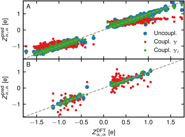
Scatter plot of diagonal components of the BECsZααcomparing DFT values with model predictions for bulk water (A) and water clusters (B).

Overall, the uncoupled and the coupled model with local screening (γi) both reproduce the BEC labels accurately for the bulk and for the clusters. The global-screening model, however, shows a clear deterioration in performance on both subsets. This stems from the global model's homogeneous-screening assumption: as expected from our discussion above, a singleγcannot simultaneously capture the different effective dielectric responses present in homogeneous bulk and inhomogeneous cluster environments. For this global-γmodel—whereγwas obtained by ana posteriorifit to the BEC labels of the validation-set—we findγ= 1.974. While one could reduce the error further by fitting distinct screening factors for bulk and cluster subsets, this strategy requires identifying and splitting the dataset into several classes based on their structure. As dataset size and diversity grow, such manual classification becomes increasingly impractical.

Furthermore, the local screening varies strongly in clusters.Fig. 3shows the distributions of local screening valuesγipredicted by the coupled local-γimodel as a function of the number of moleculesNmolper cluster. For small clusters the predictedγivalues are tightly distributed, whereas the distributions broaden as cluster size increases. Notably, we observe pronounced differences for dangling OH groups, highlighted by the color-coded structures inFig. 3A. This trend is also reflected in the bimodal distribution of hydrogen-atomγivalues in cluster structures, which we attribute to the distinction between hydrogens engaged in hydrogen bonding and those exposed at the cluster surface.

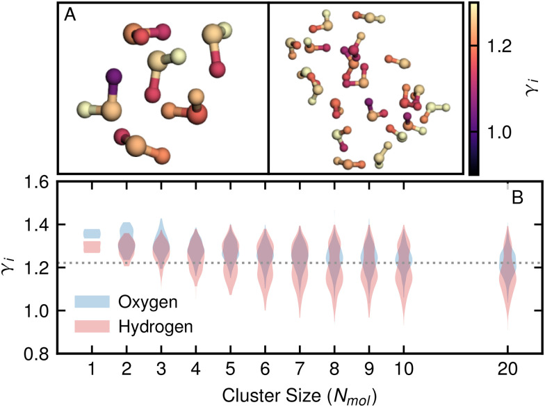
(A) Snapshot of water clusters with 6 and 20 molecules. Atoms are colored according to their local screening valuesγi. An interactive view for the whole validation set is provided onlinehttps://doi.org/10.24435/materialscloud:fs-8h. (B) Distribution of the local screening values from the coupledγimodel as a function of water cluster sizes. Gray dashed line shows the average value ofγifor bulk structures.

InFig. 3B, the dashed gray line indicates the mean screening value for bulk structures, Created by potrace 1.16, written by Peter Selinger 2001-2019 i= 1.22 ± 0.09, which theγivalues approach for larger clusters, as expected. Together, these findings provide a physically interpretable explanation for the coupling between learned pseudo charges, infrared charges, and BECs. Accurate modeling in heterogeneous environments requires this coupling to depend on the local atomic environment. By contrast, a single global screening parameter fails to capture the variability present in inhomogeneous structures.

In order to estimate the general fidelity of the different MLIP architectures, we compare the different models in terms of their mean absolute errors (MAEs) on validation sets for energies, forces and BECs (Fig. 4). Discussing first the physical models, we find differences in energy and force errors to be minor, with the uncoupled model performing overall the best. As already observed inFig. 2, the coupled globalγmodel performs significantly worse on BEC predictions, while the uncoupled and coupled localγimodels achieve similar accuracies for predicting BECs, underscoring the need for environment dependent coupling between learned pseudo charges and BECs for these systems. Importantly, modeling the coupling increases the computational cost by a constant prefactor relative to the uncoupled model, while the asymptotic scaling with system size remains unchanged (see Fig. S1 in the SI).

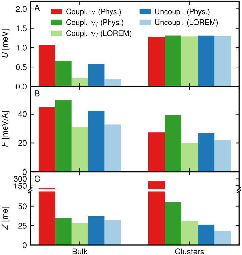
Mean absolute errors (MAE) on the validation sets for the energyU(A), forcesF(B) and the BEC diagonal elementsZ(C). Different colors depict different models. Light color bars show physical models while desaturated bars show the LOREM models.

So far, all models were trained utilizing the physically motivated Coulomb interaction ofeqn (5). To investigate if a more expressive but less physically interpretable model utilizingeqn (6)may perform even better, we also trained models with the LOREM formulation. As can be seen inFig. 4, this modification improves performance on all targets with a particularly strong improvement in bulk potential energy errors. The parity plot (similar toFig. 2) for the LOREM models are presented in the SI (Fig. S2), showing qualitative agreement with the physical models and mirroring the need for an environment dependent coupling parameter to achieve good BEC accuracy on cluster and bulk structures. However, as shown in Fig. S3, the local screening valuesγipredicted by the LOREM models are no longer physically interpretable due to the learnable mappingfθ.

Finally, we assess the behavior of the different physical models in predicting infrared spectra from molecular dynamics simulations. Computational details are provided in method Section 5.3.Fig. 5shows the imaginary part of the complex susceptibility for periodic bulk water atT= 300 K and for the cage and book configurations of water hexamer clusters atT= 10 K. The spectra are organized into two columns: the left column (panels A, C, E) shows the OH-bending mode around ∼50 THz, while the right column (panels B, D, F) shows the OH-stretching mode around ∼100 THz. We note that nuclear quantum effects are neglected, so comparison with experiment is qualitative, although error cancellation in GGA functionals yields reasonable agreement for bulk water. To contextualize the sensitivity of spectra to the predicted BECs, we also provide results for an analysis based on constant scalar charges. To this end, we calculate the average diagonal component of the BECs per element and assign this charge to all O and H atoms for the analysis of the entire trajectory. The results of this procedure are given by the purple lines inFig. 5.

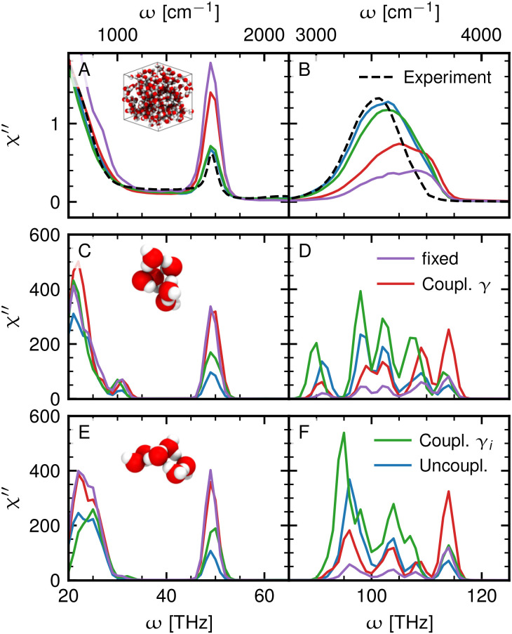
Imaginary part of the susceptibility spectrum of periodic bulk water atT= 300 K (A + B), cage (C + D) and book (E + F) configuration of water hexamer clusters atT= 10 K. We show results for the three model architectures discussed in this work and for reference the result of a simple constant scalar charge analysis (purple line). The black dashed line shows experimental bulk reference spectrum taken from ref.36.

Focusing first on a comparison of models in the bending mode in panels A, C, E, a consistent hierarchy emerges: the fixed charge model (based on atom-type averaged charges), global screening (γ), local screening (γi), and uncoupled models estimate the bending mode amplitude in decreasing order. In bulk water, where we also provide an experimental reference, this ordering is particularly evident. The globalγmodel strongly overestimates the bending intensity (A) and underestimates the stretching band (B), which is additionally shifted to higher frequencies. The fixed-charge model shows similar but slightly more pronounced deviations from the experimental reference.

In contrast, both theγiand uncoupled models reproduce intensities and peak positions much more accurately, in closer agreement with the experiment. Discussing in more detail the results for the water hexamers, we find similar but slightly less pronounced trends. As the spectral features of these isomers have been discussed extensively elsewhere,36,57,58we focus here on differences between models. Overall, all models reproduce the main spectral features, indicating consistent nuclear dynamics. Differences arise mainly in intensities and subtle frequency shifts. The bending-mode intensity again increases with decreasing model flexibility (C, E), following the same hierarchy as discussed above, while differences in the stretching region (D, F) are more subtle. The LOREM models give spectra supporting the same conclusion, as shown in Fig. S4 in the SI. In summary, these results are consistent with the model errors discussed above, in that the global screening model shows the largest deviations in predicted infrared spectra, including for the experimentally accessible bulk water case. This reinforces the conclusion that a more local treatment of the coupling between latent and dynamic charges, as realized in theγimodel, or the complete decoupling in the uncoupled model, more accurately captures the charge redistribution underlying IR activity, particularly for the OH bending/stretching part of the spectrum, where the dynamic part of BEC contributions are expected to be pronounced. At the same time, the overall spectral shape is already reasonably well reproduced even with the simplified fixed-charge analysis, indicating that IR spectra are primarily governed by the nuclear dynamics and the symmetry of vibrational modes, while still reflecting the improved physical consistency of more flexible charge-coupling schemes.

Conclusions

Machine-learned interatomic potentials increasingly attempt to incorporate long-range electrostatics and external-field coupling by introducing atom-centered static charges and, in some cases, by exploiting a physically motivated relationship between static and dynamic charges. However, an explicit assessment of whether this physical motivation enables reliable prediction of dynamical charges without explicitly training on them is lacking, and there are no systematic studies evaluating whether coupled architectures with an explicit dynamic-charge target outperform approaches that treat static and dynamic charges separately.

In this work, we systematically examine this question within models that incorporate explicit electrostatic interactions. Using water clusters and bulk water as controlled test systems—where high-quality reference data are available and long-range polarization effects are essential—we demonstrate that even in this comparatively simple setting, static charges learned as coefficients of a Coulomb term are only correlated with Born effective charges (BECs). As we show, the relationship is not captured well with a single factor across heterogeneous environments, breaking down when fitting on systems such as clusters of varying size. We show that restoring quantitative agreement within coupled models for heterogeneous datasets requires employing spatially varying screening coefficients. While this improves accuracy, it removes the anticipated simplicity of the physically constrained approach and does not provide a clear computational advantage over directly learning BECs as an independent target. In contrast, treating dynamic charges as a separate, well-defined observable yields higher accuracy, improved infrared intensities, and lower complexity.

Even though it is tempting to avoid the explicit calculation of reference BECs, especially given that observables such as IR spectra are comparatively insensitive to moderate errors in the predicted dynamical charges, our results show that measurable and systematic differences nevertheless emerge, in particular for bulk water where experimental reference data are available. In this case, models incorporating local screening or decoupled charge responses reproduce the relative intensities and peak positions more accurately than approaches based on global screening or fixed charges. Our results indicate that whenever heterogeneous datasets are considered, quantitative accuracy is strongly improved by explicit training on BECs. For these reasons, we recommend (i) using electrostatic potentials to capture long-range interactions without attributing physical meaning to static charges, which are inherently model-dependent quantities, and (ii) learning dynamic charges explicitly and independently from well-definedab initioBEC data.

Methods

Dataset construction

The bulk water structures are taken from ref.59. The water cluster structures are composed from three sources: (1) the water cluster subset of Hobza's benchmark energy and geometry data base (BEGDB),60(2) the WATER27 component of the GMTKN24 and GMTKN30 benchmark suites61and (3) dimer and trimer structures from ref.62. These sets contain very distinct geometrical structures from 1 to 20 water molecules. To extend the dataset size we performed molecular dynamics simulations for each cluster size at a temperature of 400 K for 500 ps with a 0.5 fs timestep using the universal PET-MAD model.63We combined the initial structures with the MD runs and selected 2000 structures using farthest point sampling using the PET-MAD descriptor.64

For consistent labeling of the structures, we recalculated energies, forces and BECs for all structures with DFT at the revPBE-D3 level using the CP2K package.65These calculations employed the revised Perdew–Burke–Ernzerhof (PBE) exchange–correlation functional, a DZVP-MOLOPT atom-centered basis set, and Goedecker–Teter–Hutter (GTH) pseudopotentials.

To compute BECsviafinite electric fields we start from the right-hand-side ofeqn (1), indicating that BECs can be obtained as the derivative of atomic forces with respect to externally applied fields. This relation, strictly only true in the infinitesimal limit, can be approximatedviacentral finite differences, giving us

whereEβis the magnitude of the externally applied field in Cartesian directionβandFαiis theαCartesian component of the force on atomi. This reduces the calculation of the per-atom BECs to six plus one single-point calculations in DFT, where reusing the initial wave-function guess further significantly reduces the computational cost. We show in Fig. S5 of the SI that the estimated values for the BECs from this scheme are stable across a very wide range of externally applied field strengths. To apply homogeneous external fields we use the implementation by Souzaet al.and Umari and Pasquarello66,67(see also ref.68). For production calculations, finite field strengths of 0.026 V Å−1were applied for the central finite-difference scheme ineqn (10).

Training procedure

We construct the model to output the enthalpyH, such that the total force on atomiis given byFi= −∇riH via

wherePrefis the dipole of a reference configuration which serves to obtain a consistent definition in periodic settings.15The internal energy per atomiis simply given by the sum of long and short-ranged contributionsUmodeli=Usri+Ulri. The force given by the gradient ofeqn (11)with respect toriis thus given by:

neglecting second order derivatives ofZiwith respect tori. ProvidedPis known for a reference configuration (e.g. viaanab initiocalculation for the starting structure), the enthalpyHis well-defined throughPrefduring a simulation run. This procedure is in principle similar to what has been proposed in ref.11, even though here the ambiguity in the definition ofHis made explicit. We note the absence ofPreffor the force ineqn (12), hence forces are always well-defined, even whenPis ambiguous.

Finally, training of all models is performed by constructing a typical force and energy loss functionviaanL2norm,i.e.

whereαF,αU,αBECare hyper-parameters of the learning procedure. For some experiments, we setαBECof the coupled globalγmodel to zero in order to reproduce the work in ref.34, where BECs are fitted a posteriori from learned pseudo charges. To encourage charge-neutral predictions, we include an explicit neutrality penalty in the loss function for all models. This penalty term suppresses artifacts associated with the uniform background charge inherent to Ewald-sum-based electrostatics69and is defined as

withε= 1 × 10−12a small number to ensure numerical stability andαneutralagain a hyper-parameter. Unless otherwise noted, all loss weights were set to 1.

For the short-range features, we follow the architecture described in ref.44. All models use a cutoff radius ofrc= 5.0 Å and spherical harmonics up to degree 6, with eight spherical channels. The radial dependence is represented using 32 radial basis functions, and the chemical embedding uses eight channels. We employ a cosine cutoff to ensure smooth behavior at the cutoff distance, and perform the radial expansion using basic Bernstein basis functions.70The network uses the SiLU activation function. No message passing is applied, and for each atom a single floating-point value is predicted, representing its pseudo charge.

Training is performed using the Adam optimizer with an initial learning rate of 6 × 10−5and a batch size of one structure. Optimization proceeds until the loss no longer improves significantly. For validation, we use a random 80 : 20 train–validation split.

For the training of the coupled models with global screening parameterγ, we first train the model purely on energy and force labels. Utilizing the pseudo charge predictions of this model (througheqn (3)for non-periodic structures andeqn (9)for periodic structures) we determine a singleγvalue which minimizes the absolute error on BEC predictions on the entire validation set, including clusters and bulk structures simultaneously. This value is then used for all subsequent evaluations and simulations of the model.

Molecular dynamics and IR spectra

All simulations were carried out using the atomic simulation environment (ASE).71A time step of 0.5 fs was used in conjunction with a Bussi–Donadio–Parinello thermostat72to simulate bulk water and water clusters at constant temperature and constant volume. For simulations of clusters, we removed the center of mass velocity and rotation. All results for clusters shown in the main work are obtained as the average over 95 independent simulations of 50 ps per system and model. For the bulk systems, twenty simulations of length 100 ps are used. For comparison the SI shows results for the LOREM models obtained from five independent simulations for each system and model. The polarization time derivative follows from the chain rule19

withvithe particle's velocity. The frequency-dependent complex electric susceptibility is obtained from the polarization–polarization time correlation function36

whereP(t) is calculated fromeqn (15)vianumerical integration. Using the Wiener–Khinchin theorem, we compute the dissipative imaginary partχ″ from the polarization spectrum as

whereP̃(ω) is the Fourier transform of the polarization time series and whereLtis the length in time of the polarizationP(t).

For the reference analysis method utilizing fixed charges, we use the trajectory obtained from the uncoupled model and take the averageZ̄ααof the diagonal BEC components over 50 ps per atomic species. The dipole IR spectra are then calculatedviaeqn (17)via.

Author contributions

P. L., M. C. and A. S. designed the study. P. S. implemented the method, trained the models, performed simulations and analysis. P. L. curated the datasets, created the visualizations, and assisted with implementation and simulations. M. F. L. and E. R. contributed significantly to the design of the models, with E. R. additionally supporting model training and figure design. H. S. performed the density functional theory calculations. M. C. and A. S. supervised the project. All authors contributed to the writing of the manuscript and analysis of the results.

Conflicts of interest

There are no conflicts to declare.

Acknowledgments

We thank Michelangelo Domina, Philipp Schienbein, Bingqing Cheng, Venkat Kapil and Matthias Kellner for the insightful discussions. The work of A. S. and P. S. was funded by Deutsche Forschungsgemeinschaft (DFG, German Research Foundation) under Germany's Excellence Strategy – EXC 2075/1 – 390740016 and further supported by EXC 3120/1 – 533771286. We acknowledge the support by the Stuttgart Center for Simulation Science (SimTech). H. S. was funded by the Deutsche Forschungsgemeinschaft (DFG, German Research Foundation) under SFB 1333/2 – 358283783. M. F. L. acknowledges funding from the German Research Foundation (DFG) under project number 544947822. M. C. and P. L. acknowledge funding from the NCCR MARVEL, funded by the Swiss National Science Foundation (SNSF, grant number 182892) and from the European Research Council (ERC) under the European Union's Horizon 2020 research and innovation programme (grant agreement no 101001890-FIAMMA).

Data availability

Supplementary information (SI) is available, showing additional details on the implementation of the coupled model, computational scaling analysis, results for the LOREM models and an analysis of the numerical stability for the finite difference scheme used to obtain BEC labels from DFT. See DOI:https://doi.org/10.1039/d6cp00911e.

The atomic structures used to train the models are available fromhttps://doi.org/10.24435/materialscloud:fs-8h. In the same entry we also provide a chemiscope visualization for the validation set of the water clusters for the local gamma models containing the structures, screening values and learned pseudo charges.

Code availability: the trained models, training scripts, CP2K input files to generate the dataset, and the code to reproduce this study is available on GitHub athttps://github.com/pstaerk/si_charge_learning_bec.

Associated Data

Data Availability Statement

Supplementary information (SI) is available, showing additional details on the implementation of the coupled model, computational scaling analysis, results for the LOREM models and an analysis of the numerical stability for the finite difference scheme used to obtain BEC labels from DFT. See DOI:https://doi.org/10.1039/d6cp00911e.

The atomic structures used to train the models are available fromhttps://doi.org/10.24435/materialscloud:fs-8h. In the same entry we also provide a chemiscope visualization for the validation set of the water clusters for the local gamma models containing the structures, screening values and learned pseudo charges.

Code availability: the trained models, training scripts, CP2K input files to generate the dataset, and the code to reproduce this study is available on GitHub athttps://github.com/pstaerk/si_charge_learning_bec.

References

1. Pan Y. Wang X. Zhang W. Tang L. Mu Z. Liu C. Tian B. Fei M. Sun Y. Su H. Gao L. Wang P. Duan X. Ma J. Ding M. Nat. Commun. 2022;13:3063. doi.org/10.1038/s41467-022-30766-x
2. Ciampi S. Darwish N. Aitken H. M. Díez-Pérez I. Coote M. L. Chem. Soc. Rev. 2018;47:5146–5164. doi.org/10.1039/c8cs00352a
3. Salles N. Martin-Samos L. de Gironcoli S. Giacomazzi L. Valant M. Hemeryck A. Blaise P. Sklenard B. Richard N. Nat. Commun. 2020;11:3330. doi.org/10.1038/s41467-020-17173-w
4. Unke O. T. Chmiela S. Sauceda H. E. Gastegger M. Poltavsky I. Schütt K. T. Tkatchenko A. Müller K.-R. Chem. Rev. 2021;121:10142–10186. doi.org/10.1021/acs.chemrev.0c01111
5. Schütt K. Kindermans P.-J. Sauceda Felix H. E. Chmiela S. Tkatchenko A. Müller K.-R. Adv. Neural Inf. Process. Syst. 2017;30:992–1002.
6. Thomas N., Smidt T., Kearnes S., Yang L., Li L., Kohlhoff K. and Riley P., arXiv, 2018, preprint, arXiv:1802.08219 10.48550/arXiv.1802.08219 doi.org/10.48550/arXiv.1802.08219
7. Batzner S. Musaelian A. Sun L. Geiger M. Mailoa J. P. Kornbluth M. Molinari N. Smidt T. E. Kozinsky B. Nat. Commun. 2022;13:2453. doi.org/10.1038/s41467-022-29939-5
8. Batatia I. Kovacs D. P. Simm G. Ortner C. Csányi G. Adv. Neural Inf. Process. Syst. 2022;35:11423–11436.
9. Li Z. Scandolo S. J. Chem. Phys. 2026;164:044107. doi.org/10.1063/5.0292167
10. Kapil V. Kovács D. P. Csányi G. Michaelides A. Faraday Discuss. 2024;249:50–68. doi.org/10.1039/d3fd00113j
11. Falletta S. Cepellotti A. Johansson A. Tan C. W. Musaelian A. Owen C. J. Kozinsky B. Nat. Commun. 2025;16:4031. doi.org/10.1038/s41467-025-59304-1
12. Stocco E. Carbogno C. Rossi M. Mater. 2025;11:304. doi.org/10.1038/s41524-025-01751-x
13. Veit M. Wilkins D. M. Yang Y. DiStasio, Jr. R. A. Ceriotti M. J. Chem. Phys. 2020;153:024113. doi.org/10.1063/5.0009106
14. Martin B. A. A., Ganose A. M., Kapil V., Li T. and Butler K. T., General Learning of the Electric Response of Inorganic Materials,arXiv, 2025, preprint, arXiv:2508.17870 10.48550/arXiv.2508.17870 doi.org/10.48550/arXiv.2508.17870
15. Resta R. and Vanderbilt D., Physics of Ferroelectrics, Springer Berlin Heidelberg, Berlin, Heidelberg, 2007, vol. 105, pp. 31–68
16. Spaldin N. A. J. Solid State Chem. 2012;195:2–10.
17. Dufils T. Knijff L. Shao Y. Zhang C. J. Chem. Theory Comput. 2023;19:5199–5209. doi.org/10.1021/acs.jctc.3c00359
18. Li J. Knijff L. Zhang Z.-Y. Andersson L. Zhang C. J. Chem. Theory Comput. 2025;21:1382–1395. doi.org/10.1021/acs.jctc.4c01570
19. Schienbein P. J. Chem. Theory Comput. 2023;19:705–712. doi.org/10.1021/acs.jctc.2c00788
20. Joll K. Schienbein P. Rosso K. M. Blumberger J. Nat. Commun. 2024;15:8192. doi.org/10.1038/s41467-024-52491-3
21. Bergmann N. Bonnet N. Marzari N. Reuter K. Hörmann N. G. Phys. Rev. Lett. 2025;135:146201. doi.org/10.1103/lm64-m3bn
22. Bartók A. P. Payne M. C. Kondor R. Csányi G. Phys. Rev. Lett. 2010;104:136403. doi.org/10.1103/PhysRevLett.104.136403
23. Deng Z. Chen C. Li X.-G. Ong S. P. npj Comput. Mater. 2019;5:1–8.
24. Artrith N. Morawietz T. Behler J. Phys. Rev. B:Condens. Matter Mater. Phys. 2011;83:153101.
25. Morawietz T. Sharma V. Behler J. J. Chem. Phys. 2012;136:064103. doi.org/10.1063/1.3682557
26. Yao K. Herr J. E. Toth D. W. Mckintyre R. Parkhill J. Chem. Sci. 2018;9:2261–2269. doi.org/10.1039/c7sc04934j
27. Ko T. W. Finkler J. A. Goedecker S. Behler J. Nat. Commun. 2021;12:398. doi.org/10.1038/s41467-020-20427-2
28. Gao R. Yam C. Mao J. Chen S. Chen G. Hu Z. Nat. Commun. 2025;16:10484. doi.org/10.1038/s41467-025-65496-3
29. Cheng B. npj Comput. Mater. 2025;11:1–8. doi.org/10.1038/s41524-025-01701-7
30. Loche P. Huguenin-Dumittan K. K. Honarmand M. Xu Q. Rumiantsev E. How W. B. Langer M. F. Ceriotti M. J. Chem. Phys. 2025;162:142501. doi.org/10.1063/5.0251713
31. Gross K. C. Seybold P. G. Hadad C. M. Int. J. Quantum Chem. 2002;90:445–458.
32. Reed A. E. Weinstock R. B. Weinhold F. J. Chem. Phys. 1985;83:735–746.
33. Hirshfeld F. L. Theor. Chim. Acta. 1977;44:129–138.
34. Zhong P. Kim D. King D. S. Cheng B. npj Comput. Mater. 2025;11:384.
35. Kim D. Wang X. Zhong P. King D. S. Inizan T. J. Cheng B. J. Chem. Theory Comput. 2025;21:12709–12724. doi.org/10.1021/acs.jctc.5c01400
36. Carlson S. Brünig F. N. Loche P. Bonthuis D. J. Netz R. R. J. Phys. Chem. A. 2020;124:5599–5605. doi.org/10.1021/acs.jpca.0c04063
37. Knopf D. A. Alpert P. A. Wang B. ACS Earth Space Chem. 2018;2:168–202.
38. Netz R. R. J. Phys. Chem. B. 2020;124:7093–7101. doi.org/10.1021/acs.jpcb.0c05229
39. Milani A. Castiglioni C. J. Mol. Struct. THEOCHEM. 2010;955:158–164.
40. Mulliken R. S. J. Chem. Phys. 1955;23:1833–1840.
41. Zhang L. Wang H. Muniz M. C. Panagiotopoulos A. Z. Car R. E W. J. Chem. Phys. 2022;156:124107. doi.org/10.1063/5.0083669
42. Wang L.-P. Martinez T. J. Pande V. S. J. Phys. Chem. Lett. 2014;5:1885–1891. doi.org/10.1021/jz500737m
43. Huguenin-Dumittan K. K. Loche P. Haoran N. Ceriotti M. J. Phys. Chem. Lett. 2023:9612–9618. doi.org/10.1021/acs.jpclett.3c02375
44. Rumiantsev E., Langer M. F., Sodjargal T.-E., Ceriotti M. and Loche P., Learning Long-Range Representations with Equivariant Messages, Transactions on Machine Learning Research, 2026
45. Unke O. T. and Maennel H., E3x: E(3)-Equivariant Deep Learning Made Easy, 2024
46. Schmiedmayer B. Kresse G. J. Chem. Phys. 2024;161:084703. doi.org/10.1063/5.0217243
47. Schmiedmayer B., Rittsteuer A., Hilpert T. and Kresse G., Scalar Machine Learning of Tensorial Quantities - Born Effective Charges from Monopole Models,arXiv, 2026, preprint, arXiv:2602.04773 10.48550/arXiv.2602.04773 doi.org/10.48550/arXiv.2602.04773
48. Leontyev I. V. Stuchebrukhov A. A. J. Chem. Phys. 2009;130:085102. doi.org/10.1063/1.3060164
49. Leontyev I. V. Stuchebrukhov A. A. J. Chem. Theory Comput. 2010;6:3153–3161. doi.org/10.1021/ct1002048
50. Kornyshev A. A. J. Electroanal. Chem. Interfacial Electrochem. 1986;204:79–84.
51. Stern H. A. Feller S. E. J. Chem. Phys. 2003;118:3401–3412.
52. Ballenegger V. Hansen J.-P. J. Chem. Phys. 2005;122:114711. doi.org/10.1063/1.1845431
53. Stärk P. Stooß H. Loche P. Bonthuis D. J. Netz R. R. Schlaich A. Chem. Phys. Rev. 2026;7:011319.
54. Bereau T. Andrienko D. von Lilienfeld O. A. J. Chem. Theory Comput. 2015;11:3225–3233. doi.org/10.1021/acs.jctc.5b00301
55. Langer M. F. Frank J. T. Knoop F. J. Chem. Phys. 2023;159:174105. doi.org/10.1063/5.0155760
56. Langer M. F. Knoop F. Carbogno C. Scheffler M. Rupp M. Phys. Rev. B. 2023;108(10):L100302.
57. Pérez C. Muckle M. T. Zaleski D. P. Seifert N. A. Temelso B. Shields G. C. Kisiel Z. Pate B. H. Science. 2012;336:897–901. doi.org/10.1126/science.1220574
58. Wang Y. Bowman J. M. J. Phys. Chem. Lett. 2013;4:1104–1108. doi.org/10.1021/jz400414a
59. Cheng B. Engel E. A. Behler J. Dellago C. Ceriotti M. Proc. Natl. Acad. Sci. U. S. A. 2019;116:1110–1115. doi.org/10.1073/pnas.1815117116
60. Temelso B. Archer K. A. Shields G. C. J. Phys. Chem. A. 2011;115:12034–12046. doi.org/10.1021/jp2069489
61. Bryantsev V. S. Diallo M. S. van Duin A. C. T. Goddard W. A. I. J. Chem. Theory Comput. 2009;5:1016–1026. doi.org/10.1021/ct800549f
62. Nguyen T. T. Székely E. Imbalzano G. Behler J. Csányi G. Ceriotti M. Götz A. W. Paesani F. J. Chem. Phys. 2018;148:241725. doi.org/10.1063/1.5024577
63. Mazitov A. Bigi F. Kellner M. Pegolo P. Tisi D. Fraux G. Pozdnyakov S. Loche P. Ceriotti M. Nat. Commun. 2025;16:10653. doi.org/10.1038/s41467-025-65662-7
64. Mazitov A. Chorna S. Fraux G. Bercx M. Pizzi G. De S. Ceriotti M. Sci. Data. 2025;12:1857. doi.org/10.1038/s41597-025-06109-y
65. Kühne T. D. Iannuzzi M. Del Ben M. Rybkin V. V. Seewald P. Stein F. Laino T. Khaliullin R. Z. Schütt O. Schiffmann F. Golze D. Wilhelm J. Chulkov S. Bani-Hashemian M. H. Weber V. Borštnik U. Taillefumier M. Jakobovits A. S. Lazzaro A. Pabst H. Müller T. Schade R. Guidon M. Andermatt S. Holmberg N. Schenter G. K. Hehn A. Bussy A. Belleflamme F. Tabacchi G. Glöß A. Lass M. Bethune I. Mundy C. J. Plessl C. Watkins M. VandeVondele J. Krack M. Hutter J. J. Chem. Phys. 2020;152:194103. doi.org/10.1063/5.0007045
66. Souza I. Íñiguez J. Vanderbilt D. Phys. Rev. Lett. 2002;89:117602. doi.org/10.1103/PhysRevLett.89.117602
67. Umari P. Pasquarello A. Phys. Rev. Lett. 2002;89:157602. doi.org/10.1103/PhysRevLett.89.157602
68. Stengel M. Spaldin N. A. Vanderbilt D. Nat. Phys. 2009;5:304–308. doi.org/10.1038/nmat2429
69. Barr S. A. Panagiotopoulos A. Z. Phys. Rev. E:Stat., Nonlinear, Soft Matter Phys. 2012;86:016703. doi.org/10.1103/PhysRevE.86.016703
70. Lorentz G. G., Bernstein Polynomials, American Mathematical Society, New York, NY, 1986
71. Hjorth Larsen A. Jørgen Mortensen J. Blomqvist J. Castelli I. E. Christensen R. Duak M. Friis J. Groves M. N. Hammer B. Hargus C. Hermes E. D. Jennings P. C. Bjerre Jensen P. Kermode J. Kitchin J. R. Leonhard Kolsbjerg E. Kubal J. Kaasbjerg K. Lysgaard S. Bergmann Maronsson J. Maxson T. Olsen T. Pastewka L. Peterson A. Rostgaard C. Schiøtz J. Schütt O. Strange M. Thygesen K. S. Vegge T. Vilhelmsen L. Walter M. Zeng Z. Jacobsen K. W. J. Phys.: Condens. Matter. 2017;29:273002. doi.org/10.1088/1361-648X/aa680e
72. Bussi G. Donadio D. Parrinello M. J. Chem. Phys. 2007;126:014101. doi.org/10.1063/1.2408420

---

Republished from the open web under CC-BY. Authors: Stärk P, Stooß H, Langer MF, Rumiantsev E, Schlaich A, Ceriotti M, Loche P. Read the original.